Measuring Strategic Communications

(1)

University of South Carolina

Scholar Commons

Theses and Dissertations

6-30-2016

Bayesian Semiparametric Quantile Regression for

Clustered Data

Xin Tong

University of South Carolina

Follow this and additional works at:https://scholarcommons.sc.edu/etd

Part of theOther Public Health Commons

This Open Access Dissertation is brought to you by Scholar Commons. It has been accepted for inclusion in Theses and Dissertations by an authorized administrator of Scholar Commons. For more information, please [email protected].

Recommended Citation

Tong, X.(2016).Bayesian Semiparametric Quantile Regression for Clustered Data.(Doctoral dissertation). Retrieved from

(2)

Bayesian Semiparametric Quantile Regression for Clustered Data

by

Xin Tong

Bachelor of Science Nanjing University 2007

Master of Science in Public Health University of South Carolina 2011

Submitted in Partial Fulfillment of the Requirements

for the Degree of Doctor of Philosophy in

Biostatistics

The Norman J. Arnold School of Public Health

University of South Carolina

2016

Accepted by:

Bo Cai, Major Professor

Marco Geraci, Committee Member

Alexander McLain, Committee Member

Lianming Wang, Committee Member

(3)

c

Copyright by Xin Tong, 2016

(4)

Acknowledgments

I would like to express my deep and sincere gratitude to everyone who supported and

helped me over the past few years. They have made my graduate study possible.

First and foremost, I would like to thank my advisor Bo Cai for his insightful

guidance, endless patience and invaluable advice throughout my doctoral study. This

thesis would not be possible without his constant support and inspiration make my

doctoral research productive and stimulating.

I am especially thankful to my committee members, Dr. Marco Geraci, Dr. Alex

McLain and Dr. Lianming Wang for joining my committee. I greatly appreciate

constructive feedback they have provided. I have learned a lot about the concept and

modeling methodology of quantile regression for longitudinal data by talking with

Dr. Geraci. I am very grateful to Dr. Wang for advising me with his expertise on

interval-censored data. I would like to express my gratitude to Dr. McLain for his

perpetual encouragement along the way.

The faculty of this department are very resourceful and have provided me with

a tremendous graduate education. Further thanks go to Dr. James Hussey, Dr.

Robert Moran, Dr. Jiajia Zhang for their enlightenment, which has provided me a

solid foundation to progress upon my graduate study. I also would like to thank Dr.

Suzanne McDermott for offering me a research assistantship during my PhD study.

Most of all, I thank my parents, Lianfang Tong, Yahui Wang and my husband,

(5)

Abstract

Traditional frequentist quantile regression makes few assumptions on the form of

the error distribution and thus is able to accommodate non-normal errors. However,

inference on the quantile regression models could be challenging for the unknown error

distribution, though asymptotic or resampling methods were developed. Bayesian

literature on quantile regression with random effects is relatively limited. The quantile

regression approach proposed in this dissertation is founded on Bayesian probabilistic

modeling for the underlying unknown distributions. By adopting the error density

with a nonparametric scale mixture models, we developed Bayesian semiparametric

models to make an inference on any quantile of interest and to allow for flexible shapes

of the error densities.

In this dissertation, we aimed to develop Bayesian semiparametric quantile

re-gressions for both longitudinal data and clustered interval-censored data. We first

proposed a semiparametric quantile mixed effect regression for clustered data, which

relaxed normality assumption for both random effects and the error term. We then

developed a semiparametric accelerated failure time quantile regression for the

clus-tered interval-censored data. Both of the methods allow for estimates for the subgroup

specific parameters and the detection of heterogeneity in the random effects

popu-lation under nonparametric settings. Markov chain Monte Carlo (MCMC) methods

provide computationally feasible implementations of Bayesian inference and learning.

However, the speed of convergence can be challenging for highly complex and

non-conjugate models. Specifically, Gibbs sampling algorithm that employs the addition

(6)

Sev-eral variations of the proposed model were considered and compared via the deviance

information criterion. The performance of the proposed methods was evaluated by

extensive simulation studies, and examples using data from Orthodontic clinics and

(7)

List of Tables

Table 1.1 Coefficients estimates for quantile regression and linear

regres-sion for the birth weight example . . . 10

Table 2.1 Simulation study scenarios . . . 31

Table 2.2 Simulation Results for Scenario (1) . . . 34

Table 2.3 Geweke’s Statistics for Markov Chains of the Proposed Model in Scenario (1) . . . 35

Table 2.11 Summaries and coverage probabilities of 95% intervals: compar-ing Reich’s marginal random effects model and the proposed method 45 Table 2.12 Simulation Results (a), (b), (c) . . . 48

Table 2.13 Coefficient estimates for Orthodontic data set at τ = 0.1, . . . ,0.9 . 52 Table 2.14 Quantile coefficient β0(τ = 0.5): fixed effect and random effect . . 52

(10)

Table 4.2 Geweke’s convergence diagnostic for MCMC chains of the QAFT

with Normal mixture errors . . . 83

Table 4.3 Geweke’s convergence diagnostic for MCMC chains of the

BN-QAFT with ALD errors . . . 83

BN-QAFT with Normal Mixture errors . . . 84

BN-QAFT with Normal mixture errors . . . 85

Table 4.6 Simulation Results for two models with ALD errors . . . 88

Table 4.7 Simulation Results for two models with Normal Mixture errors . . 89

Table 4.8 Geweke’s convergence diagnostic for MCMC chains of the model

parameters in the lymphatic filariasis data . . . 92

Table 4.9 Estimates of parameters in the lymphatic filariasis data . . . 92

Table A.1 Determination of precision parameters by DIC at quantile level 0.1 107

Table A.2 Determination of precision parameters by DIC at quantile level

(11)

List of Figures

Figure 1.1 Estimated parameters by quantile level . . . 10

Figure 1.2 Estimated parameter smoking by quantile level . . . 11

Figure 2.1 Using auxiliary parameters to represent conditional prior dis-tribution for a new observation. . . 28

Figure 2.2 Trace plot at quantile level 0.5 in Scenario (1) . . . 35

Figure 2.3 Trace plots of Proposed method at quantiles: 0.1, 0.5, 0.9 . . . 44

Figure 2.4 Errors of Proposed method at quantiles: 0.1, 0.5, 0.9 . . . 44

Figure 2.5 Errors comparison of Proposed method at quantiles: 0.1, 0.5, 0.9 . 46 Figure 2.6 Errors in Scenario (c) . . . 49

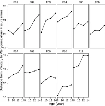
Figure 2.7 Plots of Distance against Age for each female . . . 50

Figure 2.8 Relationship between Distance and Age for each female in one plot 50 Figure 2.9 Regression quantiles for distance and 95% confidence intervals (shaded area). Least squares estimates (dashed lines) and 95% confidence intervals (dotted lines) are reported. . . 53

Figure 2.10 LQMM: Regression quantiles for distance and 95% confidence intervals (shaded area). Least squares estimates (dashed lines) and 95% confidence intervals (dotted lines) are reported. . . 53

Figure 2.11 Trace plot for each quantile level . . . 54

Figure 2.12 Error plot for each quantile level . . . 55

(12)

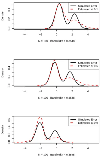
Figure 4.2 Error comparison for QAFT model with ALD errors . . . 80

Figure 4.3 Traceplots of posteriors for MCMC chains of the model

param-eters with Normal mixture errors . . . 81

Figure 4.4 Error comparison for QAFT model with Normal mixture errors . 82

Figure 4.5 Traceplots of posteriors for proposed method MCMC chains of

the model parameters with ALD errors . . . 84

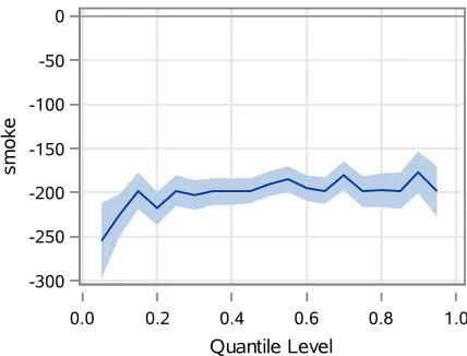
Figure 4.6 Error plot for proposed method each quantile level with ALD errors 85

Figure 4.7 Traceplots of posteriors for proposed method MCMC chains of

the model parameters with mix errors . . . 86

Figure 4.8 Error plot for proposed method each quantile level with mix errors 87

Figure 4.9 Survival curves by treatment group . . . 90

Figure 4.10 Traceplots of posteriors for MCMC chains of the model

(13)

Introduction

Linear mixed models are frequently used to describe longitudinal and repeated

mea-surements data where random effects serve to model the between-individual

correla-tion structure. One of the basic model assumpcorrela-tions of mixed model is the normality

of the random effects, which is chosen mainly for computational convenience.

How-ever, the normality assumption is typically made for the sake of convenience, rather

than from some theoretical justification, and might be inappropriate in some

situa-tions. Another troublesome fact, as noted by [Burr and Doss, 2005], is that random

effects, unlike error terms, cannot be checked (there are no residuals). Thus we are

totally dependent on this uncheckable model assumption. It is of potential interest to

model the error nonparametrically while accounting for the correlation of observations

within the same subject. Extensive work have been done on a more flexible,

possi-bly nonparametric distribution for random effects in both frequentist and Bayesian

methods, such as Dirichlet Process (DP) prior to model random effects [Bush and

MacEachern, 1996, Kleinman and Ibrahim, 1998b].

Most linear mixed models also assume that random errors are normally distributed

with constant variances. However, in some applications, the covariates may have

dif-ferent impacts at difdif-ferent locations of the response distribution. For instance, in a

birth weight study, Abrevaya and Dahl [2008] found that gender of the baby and the

mother’s prenatal-care visits have different effects at the lower and upper quantiles of

the infant birth weight distribution. In such scenarios, modeling the mean is limiting

and thus cannot accommodate population heterogeneity. Quantile regression extends

(14)

outcome variable, by allowing the tail quantiles of the conditional distribution of the

response variable as functions of a set of covariates [Koenker and Bassett Jr, 1978].

By focusing on the conditional quantiles, quantile regression offers an alternative

an-alytic tool that can automatically capture the heterogeneity in covariate effects at

different quantiles of the response distribution without modeling the

heteroscedas-ticity. Quantile regression is free from the distributional assumptions and robust to

the presence of outliers and therefore quantile regression is appropriate with skewed

distributions.

The dissertation is organized as follows. We begin with an introduction of mixed

models, quantile regression and quantile regression for longitudinal data in chapter 1.

The use of asymmetric Laplace distribution (ALD) for the error distribution provides

a natural way to deal with the Bayesian quantile regression [Yu and Moyeed, 2001],

but lacks flexibility in error distribution. [Kottas and Krnjanić, 2009] proposed an

approach to inference for nonparametric quantile regression founded on probabilistic

modeling for the underlying unknown (random) distributions. The flexibility of such

inference under nonparametric prior models is attractive and can be incorporated

into mixed models for longitudinal data. Chapter 2 presents a Bayesian

semipara-metric approach to random effects model using Dirichlet process mixtures for the error

distribution. Two simulation results are presented and indicate that the presented

approach works well for practical situations. In chapter 3, we provide an overview

of interval-censored data and two common regression models, proportional hazard

model and accelerated failure time model, and discuss some existing approaches for

regression analysis of clustered interval-censored failure time data. We are interested

to explore a flexible quantile regression framework for analysing time-to-event data

that are randomly interval-censored in chapter 4. Quantile regression models the

conditional quantiles of the survival time directly and allows the covariates to have

(15)

cap-ture important population heterogeneity [Koenker, 2005]. We adopt an accelerated

failure time model with random effects to analyze clustered interval-censored data in

the nonparametric quantile regression framework. A nonparametric Dirichlet process

prior random effects component has been used to provide flexible distributional forms

to the random effects. In addition, a Bayesian quantile regression model for clustered

interval-censored data with parametric error distribution is also constructed for

com-parison. Lastly, chapter 5 provides some discussion and offer some recommendations

on how to proceed in this Bayesian nonparametric quantile regression with random

(16)

Chapter 1 Background of Quantile Regression for

Longitudinal Data

Inference of quantile analysis has received increasing attention in recent years.

Quan-tile regression seeks to model each quanQuan-tile of the response distribution, whether

separately or jointly, conditional upon covariates. It extends regression for the mean

to the analysis of the entire conditional distribution of the outcome variable.

Regres-sion quantiles are robust against the influence of outliers [Huber, 1981], and in many

regression examples, we might expect a different structural relationship for the higher

(or lower) responses than the average responses. In such applications, mean (or

me-dian) regression approaches would likely overlook important features that could be

uncovered by a more general quantile regression analysis.

The construction of infant and adolescent growth charts provides a motivating

application of applying quantile regression to longitudinal data [Wei et al., 2006].

It is of importance to construct reference growth charts that accurately represent

the conditional quantiles of the growth distribution without unduly constraining the

estimation process by unverifiable distributional assumptions.

1.1 Mixed Models with Heterogeneity in Random Effects

Longitudinal data are characterized by repeated measurements on the same subject

over time, as may be collected in clinical trials, panel research, epidemiological

(17)

where covariate effects are modeled parametrically and with-in subject correlations

are modeled using random effects [Laird and Ware, 1982]. Letyij denote the response

for ith subject and jth repeated measurements, the random effects model for yij is

given by

yij =Xijβ+Zijbi+ij, i= 1, . . . , n, j= 1, . . . , ni, (1.1)

where the subscript i would index individual subjects, and the subscript j would

index the ni distinct measurements made on the ith subject. yij is the outcome

for the jth measure on the ith subject, Xij is a 1× p vector of fixed covariates;

β is a p×1 parameter vector of regression coefficients, β = (β1, . . . , βp)T, referred

to as fixed effects in the models; Zij is typically a subset of Xij, 1× q vector of

covariates for the q ×1 vector of random effects bi with q ≤ p, bi = (bi1, . . . , biq)T

is assumed to be normally distributed as Nq(0,D). Here D is a q ×q

positive-definite covariance matrix. ij is usually assumed to be independent and normally

distributed as Nni(0, σ2I). The random effects component Zijbi can be considered

as the deviation from the population mean Xijβ. bi is a vector of individual specific

regression coefficients, which is assumed to be independently distributed from the

error terms i. Marginalizing the random effects bi, we have

yij|β, D, σ2 ∼N(Xijβ, ZijDZijT +σ2I) (1.2)

Inference for regression parameters can be done by generalized least squares,

maxi-mum likelihood methods or empirical Bayesian method.

The dominant paradigm in the random effects literature has been a Gaussian

structure in which covariates exert a pure location shift effect on the response

vari-able. McCulloch and Neuhaus [2011] argued that misspecifying the shape of a random

effects distribution does not matter as long as the assumed distributions are not quite

far from non-normality, not as extreme as a two-point, discrete distribution,

(18)

of heterogeneity associated with the covariates under less stringent distributional

as-sumptions, while still accounting for individual specific effects. Frequentist inference

regarding fixed effects should not be much affected asymptotically by changing the

distribution of the random effects since the first two moments of the marginal

distri-bution of the response variable do not depend on the normality of the distridistri-bution

of the random effects. In equation 1.2, the individual regression coefficients simply

result in a complex covariance structure. On the other hand, bayesian inference for

fixed effects will depend on (y, σ2, D), and this dependence will be sensitive to the

distributional form ascribed to the bi [Kleinman and Ibrahim, 1998b]. Verbeke and

Lesaffre [1996] shows that random effects may be badly estimated under normal error

while the true error distribution is not normally distributed, and the current methods

for inspecting the appropriateness of the model assumptions are not sound. A more

flexible and robust approach to solve the Gaussian restricted random effect

distribu-tion problem is to use a nonparametric distribudistribu-tion, such as Dirichlet process which

will be discussed in section 1.3.1. Such model has the potential to capture more types

of variability in those effects with the possible end result of more precise estimates of

the fixed effects.

1.2 Quantile Regression

Quantile regression has been used as an attractive analytic technique to examine

many situations including risk management, portfolio optimization and asset pricing

in econometrics. The use of quantile regressions is versatile with many advantages.

It allows us to study the impact of predictors on different quantiles of the response

distribution, and thus provides a complete picture of the relationship between the

re-sponse variable and the predictors. The entire conditional distribution of the

depen-dent variable can be characterised by using different values of τ. Median regression

(19)

heteroscedasticity. Quantiles are invariant to monotonic transformations and are not

sensitive to outlier observations on the dependent variable. Finally, when the error

term is non-normal, quantile regression estimators may be more efficient than least

squares estimators since estimation and inference are distribution-free.

Basics of Quantile Regression

By extending the standard additive regression formulation, theτth quantile regression

model for (continuous) response observationsyi, with associated covariate vectorsxi,

i= 1, . . . , n, can be written as

yi =h(xi) +i (1.3)

where the i is the error term whose distribution (with density fτ(·)) is restricted to

guarantee the τth quantile of i is zero, that is R−∞0 fτ(i)di = τ. The linear model

for the τth quantile is

yi =xTi βτ +i (1.4)

where the τth quantile of i is zero. Koenker and Bassett Jr [1978] specify the τ-th

conditional quantile function as

Qτ(yi|β,xi) =xTi βτ, i= 1, ..., n

where τ ∈ (0,1), yi is a scalar response variable with conditional cumulative

distri-butionFy,Qyi(·)≡Fyi−1(·),βτ ∈Rp is a column vector of unknown fixed parameters

with lengthp. One can trace the entire conditional distribution of the dependent

vari-able, conditional on the set of predictors, by increasing τ from 0 to 1. Conditional

quantile model specifies a different model for each quantile of the outcome

distribu-tion. Interpretation of β_τ is straightforward: the intercept term simply represents

the baseline predicted quantile, while each slope can be interpreted as the rate of

change of theτth response quantile per unit change in the value of the corresponding

(20)

conditional distributions and makes no distributional assumption about the error

term in the model. However, there is no probability model for the response

distribu-tion in classical quantile regression, point estimadistribu-tion for ˆβ_τ proceeds by solving an

optimization problem of the loss function

argmin_β_∈_Rτ n X

i=1

ρτ(yi−xTi β) (1.5)

where ρτ(υ) = υ(τ −I(υ ≤ 0)) is the quantile loss function; see [Koenker and

Bas-sett Jr, 1978]. I(·) is an indicator function such that I(υ ≤ 0) = 1 if υ ≤ 0 and

I(υ ≤0) = 0, otherwise.

Asymmetric Laplace distribution provides a natural link between minimization of

the quantile loss function and maximum likelihood theory by assuming the error term

in equation (1.4) follows ALD. See [Koenker and Machado, 1999, Yu and Moyeed,

2001, Yu and Zhang, 2005] for more details. A random variableY follows an ALD if

its corresponding probability density is

f(y|µ, σ, τ) = τ(1−τ)

σ exp

−ρτ(

y−µ

σ )

(1.6)

where ρτ(·) is the loss function, σ >0 is the scale parameter and−∞< µ < +∞ is

the location parameter.

Assume yi ∼ ALD(µi, σ, τ), µi = xTiβτ. The likelihood for N independent

obser-vations is

L(β, σ,y, τ) = "

τ(1−τ)

σ

#N exp

(

−

N X

i=1

ρτ(

yi−xTi βτ

σ )

)

(1.7)

Consideringσ a nuisance parameter, the maximization of the likelihood in (1.7) with

respect to the parameter β_τ is equivalent to the minimization of the loss function

in (1.5). The relationship between the loss function and ALD can be used to

refor-mulate the quantile regression method in the likelihood framework. By utilizing this

property, [Koenker and Machado, 1999] proposed a likelihood-based goodness-of-fit

(21)

inference about the quantile regression by using asymmetric Laplace distribution to

form likelihood function, and Yu et al. [2003] studied the Bayesian estimation

proce-dure for the Tobit quantile regression model with censored data. Geraci and Bottai

[2007] and Yuan and Yin [2010] extend the asymmetric Laplace distribution idea for

longitudinal studies, which will be explained in the next section.

An Example

An example of the low birth weight study that was carried out by Koenker [2005]

will be used in this section. The data set used for this example is a subset of 50,000

observations. We are interested in investigating the relationship between infants?birth

weight (LBW: in grams) and only four predictors of interest, such as: the gender of

the infant, marital status of the mother, prenatal care, and smoking status of the

mother during pregnancy. The linear regression model for this example is:

LBW =α+β1× Gender +β2× Married +β3× Prenatal care +β4× Smoke

Linear regression is used to model the relationship between a set of predictor variable

and a response variable. It estimates the mean value of the response variable for

given levels of the predictor variables. The least square result and quantile regression

results are summarized in Table 1.1.

In each plot of Figure 1.1, the regression coefficient at a given quantile indicates

the effect on birth weight of a unit change in that variable, assuming that the other

variables are fixed, with 95% confidence interval bands.

The intercept can be interpreted as the estimated conditional quantile function of

the birth weight distribution of a girl born to an unmarried mother who didn’t smoke,

and had her first prenatal visit in the first trimester of the pregnancy [Koenker, 2005].

(22)

Table 1.1 Coefficients estimates for quantile regression and linear regression for the birth weight example

Quantile regression

Characteristic Linear regression 5th 10th 50th 90th 95th

Intercept 3224 2353 2608 3252 3856 4031

Married 161.1 227 171 149 141 165

Boy 115.9 28 84 121 142 142

Prenatal Care -227.0 -536 -418 -164 -111 -57

Smoke -200.9 -255 -226 -190 -177 -199

unmarried mother who didn’t smoke, and had her first prenatal visit in the first

trimester of the pregnancy.

According to the linear regression model,the mean weight of boys are 115.9 grams

The SAS System 13:04 Wednesday, June 17, 2015 9

The QUANTREG Procedure

With 95% Confidence Limits

Estimated Parameter by Quantile Level for weight

-600 -400 -200 0 P re na ta l_ ca re 0 50 100 150 bo y 0 50 100 150 200 250 m ar rie d 0 1000 2000 3000 4000 In te rc ep t

0.0 0.2 0.4 0.6 0.8 1.0

Quantile Level

0.0 0.2 0.4 0.6 0.8 1.0

Quantile Level

(23)

heavier than girls. But the disparity is much smaller than 100 grams in the lower tail

and larger than 120 grams in the upper tail of the distribution. The marital status

of the mother seems to be associated with a rather large positive effect on birth

weight, especially in the lower tail of the distribution. The mean weight of babies

born to mothers with no prenatal care is −227 grams lower than that of babies born

to mothers who had a prenatal visit in the first trimester. The quantile regression

results indicate that the effect of no prenatal care has a larger negative impact on

the lower quantiles of birth weight. The 5-th quantile of birth weight for infants

born to mothers who had no prenatal care is 536 grams lower than for infants born

to mothers had a prenatal visit in the first trimester. The linear regression model

underestimates this effect at the 5-th quantile. The deleterious effect of smoking is

The SAS System 13:04 Wednesday, June 17, 2015 10

The QUANTREG Procedure

With 95% Confidence Limits

Estimated Parameter by Quantile Level for weight

-300 -250 -200 -150 -100 -50 0

sm

ok

e

0.0 0.2 0.4 0.6 0.8 1.0

Quantile Level

Figure 1.2 Estimated parameter smoking by quantile level

shown in Figure 1.2. Smoking during the pregnancy is associated with a decrease of

about 160−180 grams in birth weight. The effect of smoking is quite stable over the

entire distribution, as the least-squares estimates of the mother smoking effect are

(24)

1.3 Quantile Regression for Longitudinal Data

Koenker [2004] first considered the penalized interpretation of the classical random

effects estimator in order to estimate quantile functions with subject specific fixed

effects. For a conditional quantile regression model with a random intercept, a `1

penalty is employed to shrink the random effects towards a common value. Koenker

[2004] propose to estimate αi and βτk at multiple quantile levels τk, k = 1, . . . , q by

minimizing the following penalized objective function:

q X

k=1 n X

i=1 ni X

j=1

wkρτk(yij−αi−XijTβτk) +λ n X

i=1

|αi|,

wherewk is the weight on the quantile level τk and λ is the regularization parameter

that controls the variation of αi and helps shrink bi towards a common value. As in

most regularization problems, the choice of the penalty parameter λ is crucial. For

λ→0 we obtain the fixed effect estimator by solving minα,βPqk=1

Pn

i=1 Pni

j=1wkρτk(yij−

αi−XijTβτk); while for λ→ ∞ the ˆαi →0 for all i= 1, . . . , nand we obtain an

esti-mate of the model with only the fixed effects.

As mentioned in previous section, Geraci and Bottai [2007] and Yuan and Yin

[2010] extend the asymmetric Laplace distribution idea in Yu and Moyeed [2001] for

quantile regression with independent data to clustered data, where the conditional

distribution of the response is assumed to follow an asymmetric Laplace distribution

with the mean depending on the covariates and the skewness parameter depending on

the quantile level of interest. The conditional quantile regression model includes

sub-ject specific random intercepts to account for within−subject dependence in

longitu-dinal studies. But a model with random intercepts only cannot obviously account for

between−clusters heterogeneity associated with given explanatory variables. Geraci

and Bottai [2014] propose a class of models, called linear quantile mixed models

(LQMMs), which include both random intercepts and random slopes.

(25)

j = 1, . . . , ni, i= 1, . . . , N, whereyij is the jth measurement on the ith subject. For

a given τ ∈ (0,1) ,a conditional quantile mixed model for continuous response yij is

defined by

Qyij|bi(τ|xij,bi) =x T

ijβ+z

T

ijbi (1.8)

where zij denotes a q×1 subset of covariates xij, bi is a q×1 vector of random

effects. Qyij|bi(·) is the inverse of the cumulative distribution function of the response

conditional on a location-shift random effect bi. The expression 1.8 is equivalent to

yij =xTijβ+z T

ijbi +ij (1.9)

with Qij(τ|xij,bi) = 0. The error term ij are assumed to be independently

dis-tributed as ALD and the random effect bi are also independent and follow a

multi-variate distribution. Usuallybiandij are independent of each other. The conditional

density function can be written as

f(yij|β,bi, σ) =

τ(1−τ)

σ exp

−ρτ(

yij −µij

σ )

,

where µij = xTijβ +zTijbi is the linear predictor of the τth quantile. The random

structure above allows to account for between-individual heterogeneity associated

with given explanatory variables. A recent review of linear quantile regression

mod-els for longitudinal observations is provided by Marino and Farcomeni [2015]. The

majority of the econometrics literature that studies quantile regression models for

panel data with fixed effects propose inference procedures based on the assumption

that the number of periods goes to infinity when the sample size goes to infinity. This

assumption allows to estimate unobservable fixed effects. Canay [2011] introduces a

two-step estimator for panel data quantile regression models which gets rid of the

fixed effects under the assumption that these effects are location shifters. Lamarche

[2010] elaborates the asymptotic theory of penalized quantile regression estimators

(26)

tuning parameter. Galvao [2011] studies a quantile regression dynamic panel model

with fixed effects.

Jang and Wang [2015] approximate the central density by linearly interpolating

the conditional quantile functions of the response at multiple quantiles and estimate

the tail densities by adopting extreme value theory. Through joint-quantile

model-ing, their method can yield the joint posterior distribution of quantile coefficients at

multiple quantiles and meanwhile avoid the quantile crossing issue.

1.4 Bayesian Nonparametric Modeling for Quantile Regression

Recently Bayesian nonparametric methods have been studied and developed

exten-sively, Müller and Quintana [2004] provide an overview of the respective

methodolo-gies. By modeling the response distribution and the regression function

nonpara-metrically, Bayesian nonparametric modeling provides a flexible framework for the

general regression problem. Instead of defining priors as probability distributions for

parameters in parametric Bayesian analysis, nonparametric Bayesian’s prior beliefs

are expressed as random probability measures assigned directly to the set of

proba-bility distributions. Dirichlet process (DP), which can be understood as an infinite

dimensional probability distribution over probability distributions, was originally

for-malized by Ferguson [1973] and Antoniak [1974]. And Dirichlet process mixtures are

used to model the joint distribution of response and covariates, from which full

infer-ence is obtained for the desired conditional distribution for response given covariates.

Many papers have been devoted to developing the practicality of using DP priors

[Escobar and West, 1995, MacEachern and Müller, 1998, Neal, 2000].

Yu and Moyeed [2001] propose a Bayesian approach by noting that minimizing

equation (1.5) is equivalent to maximizing a likelihood function under the asymmetric

Laplace error distribution. However, it has limitations regarding modeling skewness

(27)

level. Nonparametric error distributions based on Dirichlet process mixture models

will be discussed later in this section.

Dirichlet Process Mixture Models (DPMM)

Consider a model for joint distribution of the response,y, and the vector of covariates,

x, which in general comprises both continuous and categorical covariates. We use a

nonparametric mixture model for the joint density z= (y,x),

f(z;G) = Z

k(z;θ)dG(θ)

with a parametric kernel density k(z;θ) and a random mixing distribution G that

is modeled non-parametrically by using an infinite dimensional Bayesian model.

Fol-lowing Ferguson [1973], a distribution G on Φ follows a Dirichlet process DP(αG0)

if, given an finite measurable partition, A1, ..., Ak of Φ, the joint distribution of

(G(A1), ..., G(Ak)) is Dirichlet (αG0(A1), ..., αG0(Ak)), whereG(Ai) andαG0(Ai)

de-note the probability of setAi underGandG0, respectively. The base distributionG0

has a parametric form on Φ and E(G(A)) = G0(A). G0 acts as a prior distribution

for component parameters in the DPMM discussed later in this section. The

concen-tration or precision parameter α >0 controls the variance of the DP. As α increases,

a sampleGis more likely to be close to baseG0. A draw from the Dirichlet process is

a probability distribution. The most commonly used DP definition is its constructive

definition by Sethuraman [1994], the stick-breaking construction, which

character-ized DP realizations as countable mixtures of point masses. A random distribution

G∼DP(α, G0), then the stick-breaking representation of Gis as the following

G=

∞ X

k=1

πkδθk,

where δθk is a point mass at θk. The locations of the point passes θk arise iid from

(28)

Beta(1, α) distribution

πk =βk k−1

Y

j=1

(1−βj)

This construction emphasizes that the samples from a DP are discrete with probability

one. The term stick-breaking comes from the interpretation of mixing proportionπk;

which is given by successively breaking a unit-length stick into infinitely many pieces.

Suppose in a hierarchical model, the data zi = (xi, yi : i = 1, . . . , n) are from a

parametric distributionf with latent mixing parametersθi, a DP prior can be placed

on the parameter distribution to ensure greater model flexibility and robustness.

The general Bayesian hierarchical model by linking DP to nonparametric Bayesian

modeling can then be written as:

zi|θi ind

∼ k(zi|θi), i= 1, . . . , n

θi iid

∼ G,

G ∼ DP(α, G0)

This is often called Dirichlet process mixture model (DPMM), that we use a DP prior

on the parameter and then complete the model by introducing a likelihood.

Accord-ing to the discreteness property of the DP and its stick-breakAccord-ing representation, this

model implieszi ∼P∞k=1πkk(zi|θk), whereθkare infinite samples fromG0. Under this

formulation, the DPMM is interpreted as a flexible mixture model in which the

num-ber of components is infinite. The assumption of exchangeability [De Finetti, 1935]

makes sure that the joint distribution is invariant to the order in which observations

are assigned to clusters. Given the heterogeneity in random effects, we are also

par-ticularly interested in classifying individuals in clusters, a nonparametric Dirichlet

(29)

Subgroup Identification through Dirichlet Process

There are two schemes in clustering: one produces a hierarchical sequence of

par-titions, and the other allocates observations into proposed clusters. The latter are

based on the concept that the observations come from a heterogeneous population

consisting of several clusters. Each cluster can be modeled by a distinct

paramet-ric distribution and a mixture of these clusters, a finite mixture model, is used to

model the heterogeneity of the overall population. More explicitly, given

observa-tions y = {y1, ..., yn}, assume that there are K clusters differentiated by θk, which

can be either a scaler or a vector. Let f(·|θk) be the density of cluster k; the finite

mixture model is of the form

f(x|θ) = K X

k=1

πkf(x|θk)

withπk≥0, fork= 1, ..., K, andPKk=1πk= 1. The probabilityπkalso represents the

prior probability that an observation comes from each clusterk. One of the challenges

of using finite mixture model in clustering analysis is in determining the number of

clusters K.

The number of clusters is automatically learnt from data through DP mixture

models. DP mixtures models became popular in recent years because of the

develop-ment of simple and efficient MCMC algorithms for posterior computation

[MacEach-ern, 1994, Escobar and West, 1998, MacEachern and Müller, 1998]. It is a

generaliza-tion of mixture models to infinite components in a Bayesian framework. The P´olya

Urn scheme from Blackwell and MacQueen [1973], which most popular algorithms

rely on, integrates out the infinite dimensional G to obtain the conditional prior of

ϕi given ϕ(i) = (ϕ1, . . . , ϕi−1, ϕi+1, . . . , ϕn)0:

ϕi|ϕ(i) ∼

α

α+n−1G0+ 1

α+n−1 X

j6=i

δϕj,

(30)

ϕi equal to an element of ϕ(i) that is chosen by sampling from a discrete uniform

distribution.

The tendency of the DP to cluster subjects into groups have identical coefficients

is quite apparent from this structure. In particular, the n subjects are allocated to

K ≤ n distinct values, θ = (θ1, . . . , θK)0, with the induced prior on k stochastically

increasing withα and n [Antoniak, 1974]. Hence, although the expression is infinite,

we obtain a finite number of K clusters on integrating out the random weights and

random atoms. For this reason, DP methods are commonly used to allow uncertainty

in the number of mixture components and for clustering.

Flexible Error Distribution

Another focus in Bayesian nonparametric modeling is to find flexible error

distribu-tion. It is natural to extend a parametric class of distributions to a nonparametric

model through mixing. Kottas and Krnjanić [2009] develope two families of

nonpara-metric prior distributions based on Dirichlet process mixture models. The first model

is a general scale mixture of ALD to allow more flexible tail behavior but does not

affect the skewness of the kernel of the mixture. The second is a flexible scale mixture

of uniform densities which can capture the shape (skewness, tail behavior) of general

unimodal error densities fp(·), which is a representation of non-increasing densities

on the positive real line.

Specifically, a density fp(·) on positive real line (R+) is non-increasing if and

only if there exists a distribution function G on R+ _{such that} _f₍_t₎ _≡ _f₍_{t, G}_{) =}

R

θ−110,θ(t)dG(θ). This result can be employed to provide a mixture representation

for any unimodal density on the real line with pth quantile (mode) equal to zero,

R R

(31)

supported on R+_{, and}

kp(;σ1, σ2) =

p σ1

1(−σ1,0)() +

1−p

σ2

1_[0,σ2)() (1.10)

with 0 < p < 1, and σr > 0, r = 1,2. Assuming independent DP priors for G1 and

G2, we obtain the model for the error density R R kp(;σ1, σ2)dG1(σ1)dG2(σ2), Gr ∼

DP(αrGr0), r = 1,2. In the context of quantile regression, this model is sufficiently

flexible to capture general forms of skewness and tail behavior [Kottas and Krnjanić,

2009].

Instead of posing a parametric likelihood, Reich et al. [2010] propose to model

the likelihood nonparametrically by an infinite mixture of quantile-restricted

two-component Gaussian mixtures and to accommodate error heteroscedasticity by

speci-fying its form parametrically. They followed location-shift model with random subject

effects bi,

yij =xTijβ+bi+xTijγeij,

wherexT

ijγ >0 for allxij. They defined the random error distribution as the infinite

mixture

h(e|µ,σ2) =

∞ X

l=1

plf(e|µl,σ2l, ql),

whereplis the mixing proportion withP∞l=1pl = 1, and the base densityf(e|µl,σ2l, ql)

is the two component normal mixture

f(e|µ_l,σ_l2, ql) = qlφ(µ1l, σ12l) + (1−ql)φ(µ2l, σ22l)

where φ(µ, σ2) is the normal density with mean µ and variance σ2. The parameters

are chosen to ensureR0

−∞f(e|µl,σl2, ql)de=τ, that is, to make theτ-th quantile of e

to be zero.

Learning about the Precision Parameters

The precision parameter, α, of the Dirichlet process is extremely important for the

(32)

Whenα is large, thenGis a distribution with many support points and the

nonpara-metric model is ‘closer’ toG0, the baseline model. These features are to be borne in

mind when considering priors for α. Escobar and West [1998] discuss various effects

of the parameter α and then issues arising in learning about α within the MCMC

analysis in their book. They developed a Gibbs sampler wherein draws from the

conditional posterior distribution of α are computed by drawing successive samples

from relatively familiar distributions. In Escobar and West [1995]’s approach, prior

uncertainty in α is specified using a Gamma(a, b) distribution with fixed

hyperpa-rameters or a mixture of gamma distributions. In many cases the values of a and b

are simply varied over a range that is thought to be reasonable, Escobar and West

[1995] mentioned the possibility of using a Gamma(a, b) reference prior by letting

a →0, b→ 0. There are at two advantages of choosing a gamma prior, 1)the

distri-bution is proper so there is no need to prove posterior propriety. This is especially

important in models with many parameters where propriety may be difficult or

im-possible to prove; 2)the gamma prior leads to full conditional distributions that are

easy to sample. Gamma prior can sometimes be unstable, so a grid search should be

used to find a proper value forα.

Some researchers adopt an empirical Bayes approach wherein the maximum

like-lihood estimate (MLE) of α is computed and inferences about all other model

pa-rameters are made conditional on the MLE [Liu, 1996]. MLE of α is computed by

alternating between inference and estimation steps until convergence [Dorazio et al.,

2008]. The shortcomings are, 1) it fails to account for errors in estimating α; 2) the

empirical Bayes approach is computationally demanding, usually requiring repeated

applications of the Gibbs sampler or other Markov chain Monte Carlo algorithm; 3)

(33)

Chapter 2 A Bayesian Nonparametric Quantile Regression

for Repeated Measures with a Flexible Error

Distribution

In longitudinal studies, several repeated measurements or contaminated replicates are

often taken on the same subject with errors. Bayesian approach for the analysis of

repeated measures offers a flexible way of combining data with prior information and

inference can be always provided without the need for approximations using modern

computation methods. However, quantile regression is not equipped with a

paramet-ric likelihood, and therefore, Bayesian quantile regression for repeated measures is

challenging. As mentioned in 1.2.3, there exist several likelihood estimation methods

in parametric and semiparametric frameworks in literature. Approaches extended

from Yu and Moyeed [2001] are based on the asymmetric Laplace distribution for

the errors. Note that in ALD, the same parameter determines both skewness and

quantile level, hence limiting its flexibility in modeling skewness and tail behavior. In

this chapter, we propose a Bayesian nonparametric quantile regression for repeated

measures with error using a flexible distribution, which can capture the shape (e.g.,

skewness, tail behavior) of any unimodal error density. DP mixture models are fit

by marginalizing the random mixing distribution over its DP prior and using the

resulting Pólya urn representation for the latent mixing parameters in sampling from

the posterior.

(34)

and prior specification. Section 2.2 discusses the computational details and posterior

inference. Simulation studies to assess the performance of the proposed method are

presented in Section 2.3. An application to a data set from orthodontic clinic is

illustrated in Section 2.4. Finally, conclusions and discussion are presented in Section

2.5. The technical details are given in Appendix A.

2.1 Model Setup

Suppose we observe the data in the form (yij, Xij, Zij), i= 1, . . . , n;j = 1, . . . , ni. yij

is the jth observation of the continuous response variable on the ith subject, Xij is

thep×1 covariate vector for fixed effects, and the first covariate is one corresponding

to the intercept. For a given subject, the covariates in Xi, for instance, gender, are

assumed to remain constant across the repeated measurements. Zij is the q ×1

covariate vector for random effects. A linear mixed model has the form

yij =Xijβ+Zijbi+ij, i= 1, . . . , n;j = 1, . . . , ni, (2.1)

where β= (β1, . . . , βp)T is the unknown regression coefficient vector associated with

p model covariates, bi = (bi,1, . . . , bi,q)T are i.i.d. random effects vectors associated

with q model covariates.

To allow more flexibility in Model 2.1 we assume that the true density of the

regres-sion errors belongs to a non-parametric scale mixture of uniform densities.

Specifi-cally, A density fp(·) on positive real line (R+) is non-increasing if and only if there

exists a distribution function G on R+ such that f(t)≡f(t, G) = R

θ−110,θ(t)dG(θ).

The result on the real line with pth quantile (mode) equal to zero,

Z Z

kp(;σ1, σ2)dG1(σ1)dG2(σ2).

HereG1 and G2 are general mixing distributions, supported on R+, and

kp(;σ1, σ2) =

p σ1

1(−σ1,0)() +

1−p

σ2

(35)

with 0< p < 1, and σr >0, r = 1,2. With latent mixing parameters σ1i and σ2i for

each response, the model can be represented by

y_i, yij|β,bi, σ1i, σ2i ind

∼ kp(yij−Xijβ−Zijbi;σ1i, σ2i), i= 1, . . . , n, j = 1, . . . , ni

The likelihood becomes

n Y

i=1 ni Y

j=1

p σ1i

1(−σ1i,0)(yij −Xijβ−Zijbi) +

1−p

σ2i

1[0,σ2i)(yij −Xijβ−Zijbi) (2.3)

2.2 Prior Specification

Independent normal priors are given to fixed effect β. σ1i, σ2i are assigned

indepen-dent DP priors.

σri|Gr iid

∼ Gr, r= 1,2, i= 1, . . . , n

Gr|αr, dr ∼ DP(αrGr0), r= 1,2,

bi|Gb ∼ Gb, i= 1, . . . , n

Gb|αb, G0b ∼ DP(αbG0b)

Various noninformative prior distributions for σ have been suggested in Bayesian

literature and software, including an improper uniform density onσri [Gelman, 2006],

proper distributions such asp(σ2

ri)∼inverse-gamma. Many Bayesians have preferred

the inverse-gamma prior family, possibly because its conditional conjugacy suggested

clean mathematical properties. However, by writing the hierarchical model in the

above form, we see conditional conjugacy in the wider class of half-t distributions on

σri , which include the uniform and half-Cauchy densities on σri (as well as

inverse-gamma on σ2

ri as special cases. From this perspective, the inverse-gamma family

has nothing special to offer, and we prefer to work on the scale of the standard

deviation parameterσri, which is typically directly interpretable in the original model.

(36)

[2006], the choice of “noninformative” prior distribution can have a big effect on

inferences, especially for problems where the number of clusters (repeated measures)

is small or the cluster-level variance is close to zero. For a finite but sufficiently large

A, inferences are not sensitive to the choice of A. Random effects bi are assigned

independent DP priors. A normal base measure with zero mean is specified to G0b.

An assumed DP prior with zero mean may still imply a non-zero mean for random

effect distribution, to ensure that E(y_i) = Xiβ, the additional constraintE(bi =0)

is needed. DP precision parameters play an important role and the optimal values of

αr, r= 1,2, b are decided by the grid search.

2.3 Posterior Computation

Bayesian approach provides a flexible framework for representing the intricate nature

of the word and our knowledge of it, and the Monte Carlo methods provide a

corre-sponding flexible mechanism for inference within this framework. MCMC integration

methods, especially the Metropolis-Hastings algorithm and the Gibbs sampler have

emerged as extremely popular tools for the analysis of complex statistical models in a

short period of computers’ development. Properly defined and implemented, MCMC

methods enable users to successively sample values from values from a convergent

Markov chain, and reduce complex high-dimensional problems to a sequence of much

lower-dimensional ones. Details of MCMC methods can be found in [Geyer, 2011].

Markov Chain Sampling Methods for Dirichlet Process Mixture Models

Many different Markov chain Monte Carlo sampling techniques have been developed

for making posterior inferences from DP mixture models; Neal (2000) is a good

ref-erence. The posterior inference methods for DP mixture models we use in this study

is a combination of MCMC methods from Escobar and West [1995] and Neal [2000].

(37)

priors [Blackwell and MacQueen, 1973]. The discreteness of the DP priors [Blackwell

and MacQueen, 1973, Sethuraman, 1994] induces a clustering. We useθ= (θ1, ..., θn)

as illustrations. The most direct approach to sampling for DP mixture models is to

repeatedly draw values for each θi from its conditional distribution given both the

data and theθj forj 6=i(written asθ−i). This conditional distribution is obtained by

combining the likelihood for θi that results from yi having distribution F(θi), which

will be written as F(yi, θi) and since the observations are exchangeable, the prior

conditional on θ−i, which is

θi|θ−i ∼

α

α+n−1G0 + 1

α+n−1 X

j6=i

δ(θj)

When combined with the likelihood, this yields the following conditional distribution

for use in Gibbs sampling

θi|θ−i, yi ∼riHi+ X

j6=i

qi,jδ(θj)

Here, Hi is the posterior distribution for θ based on the prior G0 and the single

observation yi with likelihood F(yi, θ). The values of the qi,j and of ri are defined by

qi,j = bF(yi, θj)

ri = bα Z

F(yi, θ)dG0(θ)

where b is such that P

j6=iqi,j+ri = 1.

There are two main approaches for Dirichlet Process mixtures, MCMC and

vari-ational inference [Escobar and West, 1995, MacEachern and Müller, 1998, Blei and

Jordan, 2005]. Use of Dirichlet process mixture models has become computationally

feasible as the development of Markov chain methods for sampling from the posterior

distribution of the component distribution or of the associations of mixture

compo-nents with observations. In the Chinese restaurant prior, we can easily swap customer

i to the last customer to arrive by taking advantage of exchangeability, which yields

(38)

on Gibbs sampling can be easily implemented for models based on conjugate prior

distribution. Lavine and West [1992] use the Gibbs sampling approach to calculate

normal mixture models. Such iterative resampling method is applied to the mixture

model by introducing the classification variables which identify data points with

spe-cific components. However, when non-conjugate priors are used, it is often difficult to

perform numerical integration in straightforward Gibbs sampling. Later, a Markov

chain method for sampling from the posterior distribution of a Dirichlet process

mix-ture model was presented, extended Gibbs sampling for the indicators specifying

which mixture component is associated with each observation by using a set of

aux-iliary parameters [MacEachern and Müller, 1998, Neal, 2000]. The method is simple

to implement and more efficient than previous ways of handling general Dirichlet

process mixture models with non-conjugate priors. Blei and Jordan [2005] presented

a variational inference algorithm, which is a class of deterministic algorithms that

convert inference problems into optimization problems.

Gibbs Samplig Algorithm with Auxiliary Parameter

MacEachern and Müller [1998] devised an approach to handle non-conjugate priors

that uses a mapping from a set of auxiliary parameter to parameters in use. Models

with non-conjugate priors can be handled by applying Gibbs sampling to a state

that has been extended by the addition of auxiliary parameters [Neal, 2000]. In

this approach, the auxiliary parameters are regarded as existing only temporarily;

this allows more flexibility in constructing algorithms. The permanent state of the

Markov chain will bex, but a variableywill be introduced temporarily and discarded

during Markov chain simulation. The implementation of our DP is performed using

a modified algorithm proposed in Neal [2000] (Algorithm 8), which is appropriate for

models with no closed form solutions and therefore applies Gibbs sampling with the

(39)

Let ci indicates the “latent class” associated with observation yi, with the

num-bering of the ci being of no significance. We can use this technique to update ci

for a Dirichlet process mixture model without having to integrate with respect G0.

The permanent state of the Markov chain consist of c = (c1, ..., cn) and φ = (φc :

c ∈ {c1, .., c2}). For each class, c, the parameters φc determine the distribution of

observations from that class; all such φc is denoted by φ When ci is updated, we

will introduce temporarily auxiliary parameters that represent potential values for θ

that are not associated with any other observations. We then update ci by Gibbs

sampling with respect to the distribution that includes these auxiliary parameters.

Figure 2.1 represents the conditional prior distribution for a new observation using

auxiliary parameters. In this setup, the number of auxiliary parametersm = 3. The

component for the new observation is chosen from among the four components

as-sociated with other observations plus three possible new components (m = 3), with

parameters,φ5, φ6, φ7, drawn independently fromG0. The probabilities used for this

choice are shown at the top. The probability of ci being equal to a c in {1, . . . , k−}

will ben−i,c/(n−1 +α), wheren−i,c is the number of timescoccurs among thecj for

j 6=i. The probability of ci having some other value will be α/(n−1 +α), which is

split equally amongm= 3 components introduced. The dashed arrows illustrate the

possibilities of choosing an existing component, or a new component that uses one of

the auxiliary parameters in the figure.

To perform a Gibbs sampling update forci in this representation of the posterior

distribution, ci must be either one of the components associated with other

obser-vations or one of the auxiliary components that were introduced, we can easily do

Gibbs sampling by evaluating the relative probabilities of these possibilities. Once a

new value forci has been chosen, we discard all φ values that are not now associated

with an observation.

(40)

Figure 2.1 Using auxiliary parameters to represent conditional prior distribution for a new observation.

{c1, . . . , cn}). The algorithms can be summarized by repeated sampling as follows:

• For i = 1, . . . , n :, let k− be the number of distinct cj for j 6= i, and let

h = k− +m. Label these cj with values in {1, . . . , k−}. If ci = cj for some

j 6=i, draw values independently fromG0 for those φc for whichk− < c≤h. If

ci 6=cj for all j =6 i, letci have the label k−+ 1, and draw values independetnly

fromG0 for thoseG0 for thoseφc for whichk−+ 1< c ≤h. Draw a new value

for ci from {1, . . . , h} using the following probabilities:

P(ci =c|c−i, yi, φ1, . . . , φh) = 

  

  

b n−i,c

n−1+αF(yi, φc) for 1≤c≤k

−_,

b_nα/m₋₁₊_αF(yi, φc) for k−≤c≤h

(2.4)

where n−i,c is the number of cj for j 6= i that are equal to c, and b is the

appropriate normalizing constant. Change the state to contain only those φc

that are now associated with one or more observation.

• For all c∈ {c1, . . . , cn}: Draw a new value from φc|yi such that ci =c by using

the Metropolis-Hastings algorithm toφc that leaves this distribution invariant.

The posterior distributions forσri and bi can be handled by applying Gibbs

sam-pling with auxilliary parameters described in this section. The likelihood of i-th

(41)

assume both β and bi are “known”. By placing a Uniform distribution to base

dis-tribution Gr0, the conditional distribution for σri is

p(σri|yi, Gr0) ∝

αr

αr+n−1

Unif(dr)F(yi, σri) +

1

αr+n−1 X

g6=i

δ(σrg)F(yi, σri)

For each bi, suppose a Multivariate normal hyperprior for base distribution G0b

is Np(0, D), the conditional distribution

p(bi|yi) ∝ prior(bi|D)L(yi|bi)

∝ Np(0, D)p(yi|β,bi, σ1i, σ2i)

∝ 1

(2π)1/2 _|_D_|1/2exp −

1

2(bi−0) T

D−1(bi−0)

! × ni Y j=1 p σ1i

1(−σ1i,0)(yij−Xijβ−Zijbi) +

1−p

σ2i

1[0,σ2i)(yij −Xijβ−Zijbi)

Bayesian Computing for Other Parameters

Updating fixed effects β requires Metropolis-Hastings algorithms as full

condition-als distributions are not recognizable. Suppose the prior is a multivariate normal

distribution Np(0,Σ0), the conditional distribution of β is

p(β|yi) ∝ Np(0,Σ0) n Y

i=1

p(yi|β,bi, σ1i, σ2i)

∝ 1

(2π)1/2 _|_Σ 0 |1/2

exp − 1

2(β−0) T_Σ−1

0 (β−0)

! × n Y i=1 ni Y j=1 p σ1i

1(−σ1i,0)(yij −Xijβ−Zijbi) +

1−p

σ2i

1_[0,σ2i)(yij −Xijβ−Zijbi)

For the (t)-th iteration, update β by using the following Metropolis-Hastings

algo-rithm. Draw β∗ from the proposal distribution Np(βt−1, T0), and take

βt=

      

β∗ with probability min(r,1),

βt−1 with probability1-min(r,1),

(2.5)

where

r= p(β

∗_|

Measuring Strategic Communications

University of South Carolina

Scholar Commons

Bayesian Semiparametric Quantile Regression for

Clustered Data

Xin Tong

Acknowledgments

Abstract

Table of Contents

List of Tables

List of Figures

Introduction

Chapter 1

Background of Quantile Regression for

Longitudinal Data

Basics of Quantile Regression

An Example

Dirichlet Process Mixture Models (DPMM)

Subgroup Identification through Dirichlet Process

Flexible Error Distribution

Learning about the Precision Parameters

Chapter 2

A Bayesian Nonparametric Quantile Regression

for Repeated Measures with a Flexible Error

Distribution

Gibbs Samplig Algorithm with Auxiliary Parameter

Bayesian Computing for Other Parameters