R E S E A R C H
Open Access
Asymptotic equivalent analysis of the LMS
algorithm under linearly filtered processes
Markus Rupp
Abstract
While the least mean square (LMS) algorithm has been widely explored for some specific statistics of the driving process, an understanding of its behavior under general statistics has not been fully achieved. In this paper, the mean square convergence of the LMS algorithm is investigated for the large class of linearly filtered random driving processes. In particular, the paper contains the following contributions: (i) The parameter error vector covariance matrix can be decomposed into two parts, a first part that exists in the modal space of the driving process of the LMS filter and a second part, existing in its orthogonal complement space, which does not contribute to the performance measures (misadjustment, mismatch) of the algorithm. (ii) The impact of additive noise is shown to contribute only to the modal space of the driving process independently from the noise statistic and thus defines the steady state of the filter. (iii) While the previous results have been derived with some approximation, an exact solution for very long filters is presented based on a matrix equivalence property, resulting in a new conservative stability bound that is more relaxed than previous ones. (iv) In particular, it will be shown that the joint fourth-order moment of the decorrelated driving process is a more relevant parameter for the step-size bound rather than, as is often believed, the second-order moment. (v) We furthermore introduce a new correction factor accounting for the influence of the filter length as well as the driving process statistic, making our approach quite suitable even for short filters. (vi) All statements are validated by Monte Carlo simulations, demonstrating the strength of this novel approach to independently assess the influence of filter length, as well as correlation and probability density function of the driving process.
Keywords: Adaptive gradient-type filters, Mismatch, Misadjustment
1 Introduction
The well-known least mean square (LMS) algorithm [1] is the most successful of all adaptive algorithms. In its nor-malized version (NLMS), it can be found by the million in electrical echo compensators [2], in telephone switches, and also in the form of adaptive equalizers [3]. No other adaptive algorithm has been so successfully placed in commercial products.1With a fixed step-size, starting at initial valuew0, the LMS algorithm is given by
ek =dk−ukTwk =vk+ukT(w−wk) (1) wk+1 =wk+μukek ;k=0, 1, 2, . . (2)
Correspondence: [email protected]
A conference version containing preliminary results has appeared at EUSICPO conference 2011.
TU Wien, Institute of Telecommunications, Gusshausstr. 25, 1040 Vienna, Austria
Here, a reference model dk = wTuk + vk has been
introduced, as is common for a system identification prob-lem, assuming that an optimal solution w ∈ IRM×1
exists. It is further assumed that the observed system output is additively disturbed by real-valued, zero-mean, noise vk ∈ IRof variance σv2. The regression vector is uk ∈ IRM×1, with M denoting the order of the filter.
The algorithm starts with an initial value ofw0, trying to improve its estimatewk ∈IRM×1with every time instant
k. All signals are formulated as real-valued (i.e., ∈ IR), which makes the derivations easier to follow. Although, in most cases, it is straightforward to extend the results to complex-valued processes if difficulties arise, results for the complex-valued case will be pointed out.
While deterministic approaches have provenl2 stabil-ity for any kind of driving signaluk [4–7], results from
stochastic approaches are restricted to specific classes of
random processes (unfiltered independent identically dis-tributed (IID) [8], Gaussian [9, 10], and spherically invari-ant random processes (SIRP) [11]). A recent historical overview is provided in [12]. Nevertheless, such stochas-tic analysis is useful since it provides information about how the speed of convergence and the steady-state error depend on the step-sizeμ. The resulting stability bounds [8–11, 13] are typically conservative:
μclassic≤ 2 3tr[Ruu]
(3)
and are based on fourth-order moments of Gaussian vari-ables, which in turn can be expressed as second-order moments of the autocorrelation matrixRuu=EukukT
. Furthermore, the derivation of this bound for stability in the mean square sense is based on the so-called indepen-dence assumption (IA), an assumption that also will be applied throughout this article.
In Section 2, it is demonstrated that an initial parame-ter error vector covariance matrix is forced by the LMS algorithm to remain a member of the modal space ofRuu. However, this rule is not true in a strict sense for arbitrary driving processes and requires some mild approximations to make it a more general statement.
In Section 3, our considerations are complemented by analyzing the steady-state behavior of the algorithm and finally we link all these elements to a strong statement about a large class of linearly filtered random processes of the moving average type. This class naturally includes linearly filtered IID processes but it is even possible to include some particular statistically dependent terms, meaning that SIRPs are also covered. A crucial parameter to describe dynamical as well as stability behavior turns out to be the joint fourth-order momentm(x2,2)=E
x2kx2l; forl=kof the corresponding decorrelated (white)2 driv-ing process. In the case of very long filters, it turns out that even the mild approximations of the driving process are no longer required and thus less conservative step-size bounds are obtained. This is reported in Section 4. Finally, a validation of the theoretical statements is provided in Section 5 by Monte Carlo simulations. Some conclusions in Section 6 round up the paper.
Notation: To further facilitate the reading of the article, a list of commonly used variables and terms is provided in Table 1. The notation A[xk] is used to describe a
lin-ear operator on a scalar input andA[xk] on a vector input.
As the linear operator A[·] in our contribution is lim-ited to a linear time-invariant filter, it can equivalently be described by a convolutionA[xk]= Pm=0amxk−m with
the coefficients am describing the impulse response of
the filter. Consequently, A[xk]=
P
m=0amxk−m.
Equiv-alently, such a convolution can be described by a linear transformation applying an upper right Toeplitz matrix
A ∈ IRM×(M+P) to an input vector xk ∈ IR(M+P)×1.
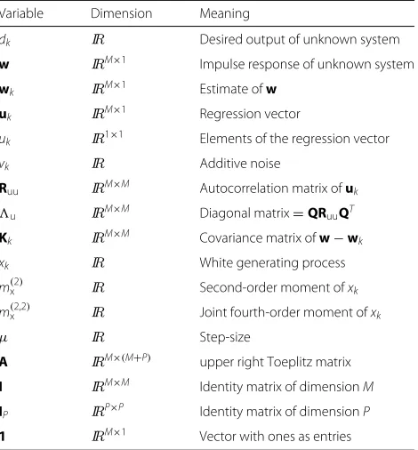
Table 1List of commonly used terms for filters of lengthM
Variable Dimension Meaning
dk IR Desired output of unknown system
w IRM×1 Impulse response of unknown system
wk IRM×1 Estimate ofw
uk IRM×1 Regression vector
uk IR1×1 Elements of the regression vector
vk IR Additive noise
Ruu IRM×M Autocorrelation matrix ofuk
u IRM×M Diagonal matrix=QRuuQT
Kk IRM×M Covariance matrix ofw−wk
xk IR White generating process
m(x2) IR Second-order moment ofxk
m(x2,2) IR Joint fourth-order moment ofxk
μ IR Step-size
A IRM×(M+P) upper right Toeplitz matrix
I IRM×M Identity matrix of dimensionM
IP IRP×P Identity matrix of dimensionP
1 IRM×1 Vector with ones as entries
In this case, the output vector uk = Axk is of
dimen-sion IRM×1. If the vectorxk =[xk,xk−1,. . .xk−M−P+1]T exhibits a shift property, so does the corresponding out-putuk =[uk,uk−1,. . .suk−M+1]T. The variablexkwill be
denoted for describing a white process throughout the paper whileukwill denote the corresponding filtered
pro-cess throughout this paper. Furthermore, two other linear operators on square matrices will be used: (1)=diag[L] on a matrixLresults in a diagonal matrixwhose diago-nal entries are identical to the diagodiago-nal ofLand all other entries are zero; (2) tr[L] on a matrix L results in the trace of the matrix, i.e., tr[L]=Mm=1Lmm. The symbol⊗
denotes a tensor or Kronecker product.
2 Modal space of the LMS algorithm
Let us consider the classical LMS analysis [8, 10], utilizing the IA as stated in the introduction:
Independence assumption (IA): The regression vectoruk
is statistically independent of the past regression vectors, i.e.,{uk−1,uk−2,. . .,u0}.
This assumption was introduced by Ungerboeck [8] and thoroughly investigated by Mazo [14] in the con-text of adaptive equalizers. A consequence of such an assumption is that parameter estimate wk (as well as
parameter error vector w˜k = w−wk) is independent
of uk and thus E
ukukT(w−wk)(w−wk)TukukT
=
EukukTE
(w−wk)(w−wk)T
ukuk
=EukukTKkukukT
where the parameter error vector covariance matrix
Kk =E
(w−wk)(w−wk)T
was applied.3In the literature, w˜
k is also often referred
to as weight error vector,wk as weight estimate, andKk
as weight error vector covariance matrix. The IA holds exactly for the linear combiner case in which the suc-ceeding regression vectors are statistically independent of each other (see, for example, in multiple sidelobe canceller (MSLC) applications [15]) while in practice, the LMS algo-rithm is mostly run on transversal filters in which the regression vectors exhibit a shift dependency. Note that we will consider the shift structure of the regression vector that isuk =[uk,uk−1,. . .,uk−M+1]T only for its genera-tion process, as it will be generated by linearly filtering random processes over time. The IA in the derivations for analyzing the algorithm will however be required which is not a contradiction to the generation process. The major advantage of the IA is that the evolution of the parameter error covariance matrixKkcan be computed and thus the
learning curves of the algorithm, i.e., its learning behavior, can be derived. This knowledge also provides the steady-state values and, furthermore, the derivation of practical step-size bounds.
Note that some analyses in the past have attempted to overcome the independence assumption; good overviews on techniques can be found in [16, 17]. In [17, 18], the authors have assumed small step-sizes (much smaller than the largest possible step-size) so that the updates are mostly static compared to the rapid changes in the sig-nals. This approach, however, basically leads to first-order results as the LMS algorithm then behaves similarly to the steepest decent algorithm. In [19, 20], Douglas et al. solved the problem by introducing a linearly filtered mov-ing average (MA) process and formulatmov-ing all terms in the evolution of the covariance matrixKkexplicitly. While the
outcomes obtained are precise, the method relies on sym-bolic computation (MAPLE) and results, even for small problems (filter orderM< 10), in a very large set of lin-ear equations. The method only provides numerical terms that neither give much insight into the functionality of the algorithm nor provide general analytical statements. Also, the approach in [21, 22] follows along such lines, however with imposing the IA, where a large set of linear equations (of the orderM2×M2) is required to be computed due to terms of the formukuTk ⊗ukuTk and then analyzed.
Simi-lar to the previous idea, this method also does not provide analytical insight and becomes tedious if not infeasible for correlated signals as well as large matrices. Finally, But-terweck [18, 23–25] has introduced a novel idea based on wave propagation. He showed that for very long fil-ters (M→ ∞), the derivation does not require the classic IA. However, several other signal conditions are required (e.g., Gaussian driving process, small step-size, infinite filter order M). Our results in Section 4 will be com-pared to his results when stability conditions for very long filters are derived. Finally, it should be mentioned that
neither do the deterministic approaches [4, 5, 7] require the IA in order to derive step-size bounds, but as in the case of other contributions, they are unable to provide learning curves or steady-state values without imposing the IA. Experimental results have shown that utilizing the IA in FIR filter structures may lead to poor learning behavior estimates under strongly correlated processes but surprisingly accurate values for steady-state values of the parameter covariance matrix. The IA therefore is still frequently used in current analyses of gradient-type algo-rithms, see, for example, recent publications [3, 26, 27]. Note that our analysis is also based on an infinite filter length approach but different to others, we quantify the error term related to the filter length which allows us to provide rather accurate results even for short filters (e.g., M=10).
In this paper, the classic stochastic approaches from Horowitz and Senne [9] and Feuer and Weinstein [10] are pursued and extended in numerous directions, relying on a general MA driving process similar to that proposed in [19, 20]. Symmetric matrices as they appear in the form of the parameter error vector covariance matrixKk can be
decomposed into two complementary subspaces (see [28] and Appendix 1 for details), namely
Kk =b0I+b1Ruu+. . .+bM−1RuuM−1+K⊥k =P(Ruu)+K⊥k.
(5)
Here, P(Ruu) denotes a polynomial in Ruu andK⊥k is an element of its orthogonal complement, i.e., every-thing inKkthat cannot be approximated byP(Ruu). Note that the impact of the complement space is only evident in the trace but not in the matrix itself: K⊥kRluu = 0
while trK⊥kRluu = 0. It turns out that only members in subspaceP(Ruu) contribute to the error performance measures (see Eq. (42) for mismatch: trKkR0uu
; see (43) for misadjustment: tr [KkRuu]) of the algorithm as only
terms of trKkRluu
are of interest while the complemen-tary part trK⊥kRluu= 0 and thus does not contribute to the performance measures.
In a first step, the following equation
K1=E
I−μu0uT0 K0
I−μu0uT0 T
=K0−μRuuK0−μK0Ruu+μ2E
u0uT0K0u0uT0
+μ2R uuσv2
(6)
is obtained. Let us start with an example to illustrate its behavior.
also allows the description of the evolution of the indi-vidual components; starting with Kk = Kk +K⊥k, with Kk∈RuandK⊥k ∈R⊥u, a set of equations is obtained
Kk+1=Kk−μRuuKk−μKkRuu
+μ22R
uuKkRuu+Ruutr
KkRuu +μ2Ruuσv2.
(7)
K⊥k+1=Kk⊥−μRuuK⊥k −μK⊥kRuu+2μ2RuuK⊥kRuu. (8)
Parameter error covariance matrixKk =Kk+K⊥k thus
evolves into a new matrixKk+1=Kk+1+K⊥k+1in which its partKkfromRustays in the modal space and appears as new part Kk+1, contributing to learning performance terms. Similarly, the perpendicular termK⊥k stays in the complement space asK⊥k+1and will thus not contribute to the algorithm’s performance curves under the trace oper-ation. The noise contributes only to the modal space. This makes it possible to formulate an initial first statement for Gaussian driving processes.
Lemma 2.1.Assume the driving process to be a corre-lated Gaussian process with autocorrelation matrixRuu.
Under the IA, the initial parameter error vector covariance matrixK0of the LMS algorithm evolves (1) into a polyno-mial inRuu of the modal space ofRuu, solely responsible
for the mismatch and the misadjustment of the algorithm, and (2) a part in its orthogonal complement which has no impact on the performance measures.
Note that the correlated Gaussian case has been solved for a while [9, 10], typically resulting in a matrix evolu-tion as presented in (7), see, e.g., [13, 29]. However, the term ((8) has never been studied at all. Including uncorre-lated IID or SIRP processes required modifications of the method [11, 30]. With the proposed method, we will be able to include arbitrary correlated processes within the same framework.
As such example presented above is somewhat intuitive for the particular case of a Gaussian driving process, what can be said about larger classes of driving processes is of interest. To achieve this goal, a number of considerations with respect to the driving process are required.
Driving process: The properties of Lemma 2.1 are not only maintained by Gaussian random processes but also by a much larger class of driving processes. It will be shown that these properties hold for random processes that are constructed by a linearly filtered white zero-mean random processuk=A[xk]=mP=0amxk−m, whose only
conditions are that:
Driving process assumptions (A1a):
m(x2) = Ex2k=1 (9)
m(x2,2) = Ex2kx2l≤c2<∞;k=l (10)
m(x4) = Ex4k≤c3<∞ (11)
m(x1,1,1,1) = E[xkxlxmxn]=0;k=l=m=n (12)
m(x2,1,1) = Ex2kxmxn
=0;k=m=n (13)
m(x1,3) = Exkx3l
=0;k=l (14)
mx = E[xk]=0. (15)
Note that the conditions are shown for real-valued pro-cesses; for complex-valued processes, they need to be adjusted. The last four conditions (12)–(15) are listed here for completeness. They exclude processes that do not have a zero mean in some sense and have been assumed, although not often explicitly mentioned, in most of the literature. Linearly filtering such processes will preserve the zero-mean properties (12)–(15). These pro-cesses certainly include not only real-valued Gaussian and SIRP 3m(x2,2)=m(x4)=3 and complex-valued
Gaus-sian and SIRP 2m(x2,2)=m(x4)=2 , processes, but also
IID processes
m(x2,2)=
m(x2) 2
. Once vectors xk =
[xk,xk−1,. . .,xk−N+1]T have been constructed, the fol-lowing second- and fourth-order expressions are found:
ExkxTk
= IN, (16)
E
xkxTkxkxTk
= m(x4)+(N−1)m(x2,2) IN. (17)
Correspondingly, the linearly filtered vectors read
uk =Axk = ⎡ ⎢ ⎢ ⎢ ⎣
a0 a1 . . . aP
a0 a1 . . . aP
. .. . .. a0 a1 . . . aP
⎤ ⎥ ⎥ ⎥
⎦xk (18)
with an upper right Toeplitz matrixAof dimensionM× N =M×(M+P). The impulse response of the coloring filter is given by a0,a1,. . .aP and appears on every row
ofAstarting witha0on its main diagonal. In general, the driving process vectorxkis longer thanuk, depending on
the orderPof the impulse response.
However, in order to guarantee independence of vectors
uk,uk−1,. . .we have to impose a second condition on the driving process:
Driving process assumptions (A1b): Assume the driving processukbeing generated by a linearly filtered processxk
as described above. We furthermore have to assume that at each time instantk, a new statistically independent pro-cess
x(lk)
time instantsk1andk2, we assume that their joint pdfs are
Note that Assumption A1b is sufficient to avoid the IA but not required. On the other hand, dropping A1b requires the IA to ensure the results of the paper hold. To facilitate reading, we will drop the notationx(lk) →xl.
With such assumptions, we are now ready for our first general statement.
Lemma 2.2.Assume driving process uk =A[xk]to
orig-inate from a linearly filtered white random process xk so
thatuk=Axkwithxk =[xk,xk−1,. . .,xk−N+1]T, whereA denotes an upper right Toeplitz matrix with the correlation filter impulse response and xk satisfies conditions (9)–
(17). The initial parameter error vector covariance matrix
K0 = K0 +K⊥0 of the LMS algorithm essentially (with error of orderO(μ2)) evolves into a polynomial inAAT
in the modal space of Ruu while terms in its orthogonal
complementK⊥either remain there or die out.
Note that this formulation may imply that this is only true for linearly filtered processes of the moving aver-age (MA) type. As no condition on the orderP of such a process is imposed, P (and thus N = M + P) can become arbitrarily large (e.g.,P → ∞) and thus autore-gressive processes (AR) or combinations (ARMA) can also be resembled as well (e.g., see [13] (chapter 2.7)).
Proof.The proof proceeds in two steps: first, rewriting (6) forK0 = Iin order to discover the most important terms and mathematical steps based on a simpler formu-lation and then refining the arguments for arbitrary values ofKktoKk+1.
Due to properties (9)–(17) of driving processxk ∈IR
E
is found, where diag[L] denotes a diagonal matrix with the diagonal terms of a matrixLas entries. Whenxk ∈CI, a
slightly different result is obtained:
ExkxkHLxkxkH
=m(x2,2)L+mx(2,2)tr[L]IM+P +m(x4)−2m(x2,2) diag[L] . (22)
For spherically invariant random processes (including Gaussian), the termm(x4)−3m(x2,2) for real-valued
sig-nals, or
m(x4)−2m(x2,2) for complex-valued signals, van-ishes and thus the problem can be solved classically.
In our particular case, L = ATA ∈ R(M+P)×(M+P)
with tr[ATA]= MPi=0|ai|2 and diag[AAT]=
P
i=0|ai|2IM+P = M1tr[ATA]IM+P. There still remains
one problematic term, however: diag[ATA]. At this point, the following is proposed:
Asymptotic equivalence: limM→∞M1 diag[ATA]−
tr[ATA]
M IM+PF = 0 with an identity matrixIM+P of the
corresponding dimension. Note that the equivalence would hold exact even for small dimensions if it had the term diag[AAT] instead of diag[ATA]. The asymp-totic equivalence can be interpreted as replacing each of the diagonal elements ofATAby their average value
1
Mtr[ATA]. Consider the relative difference matrix
= at the beginning and end of the diagonal remain unequal to zero while those terms in the middle (whose range can be substantially large ifM > P) are zero. The firstP ele-ments on the diagonal are, for example, given by,ii =
−P
m=i|am|2/Pm=0|am|2;i = 1..P. IfM P, the next
elements are all zero and finally, the lastP elements are the first in backward notation. In caseP >M/2, the zero elements do not occur. We can conclude from the con-struction of the diagonal elements,iithat they are all in
the interval(−1, 0], or alternatively ∞≤1, where we have applied a max norm. Note that for white processes a0=1 andai=0;i=1, 2,. . ., thus ∞=0.
can therefore be interpreted as being along the same lines of approximations, only originating from a different approach. We however are able to quantify the error term which will further be helpful. Note that in Section 4, this approximation will be dropped entirely for large values of Mfor different reasons. With this error term for real-valued driving processes,
is obtained with a newly introducedpdf shapecorrection value
a value that depends on the statistic of random process xk. The term m
(4)
x m(x2,2) −
3 is similar to the excess kurtosis
E|x−mx|4
2 − 3. Processes with negative
excess kurtosis are often referred to as sub-Gaussian pro-cesses while a positive excess kurtosis leads to so-called super-Gaussian processes. This (slightly abused) termi-nology will be used correspondingly to discriminate the term m(x4)
m(x2,2)−
3. Thus, sub-Gaussian processes in this sense take onγx values smaller than one while super-Gaussian processes have values larger than one. However, it is also noted that our approximation erroronly has an impact when γx = 1, which vanishes not only for Gaussian pdfs but also with decreasing step-sizeμ (which comes along naturally with growing filter orderM). If compar-ing the approximation term(γx−1)mx(2,2)tr[ATA]with γxm(x2,2)tr[ATA]IM+P, we recognize that the
approxima-tion is of order 1/Msmaller, thus diminishes with higher filter order.
Note further that the term in the LMS algorithm where the asymptotic equivalence applies is proportional toμ2. It thus has no impact for small step-sizes but certainly is expected to have one on the stability bound. A first con-clusion, therefore, is that the error on the parameter error vector covariance matrix due to this approximation is of order O(μ2). Note that the step-size being small is not to be interpreted as small relative to the step-size at the stability bound but small in absolute terms, i.e.,μ 1, which is certainly given for long filters asμ ∼ 1/M. The consequence that the applied approximation is negligible for small step-sizes (large filter order M) as well as for
Gaussian-type processes is reflected in Lemma 2.2 by the wording “essentially.” This means that in extreme cases (large μ(smallM) and far from Gaussian), a very small proportion can indeed leak into the complementary space. At the first update withK0=I,
K1 = I−2μAAT+2μ2m(x2,2)(AAT)2 (26)
+μ2m(2,2)
x γxtr[ATA]AAT+μ2AATσv2+O(μ2)
is obtained, a polynomial inAAT.
Now, the proof starts for general updates from Kk to Kk+1. While the first terms that are linear inμare straight-forward, the quadratic part inμneeds further attention.
EukukTKkukukT
Here, the same asymptotic equivalence concept as used above is imposed, i.e., diagATKkA
This can now be split into two parts, one in its modal spaceK and in its orthogonal complementK⊥as in (7) and (8) above, and the following is obtained:
Kk+1=Kk−μAATKk−μKkAAT (30)
process to remain only in the modal space of the latter. This is not only true for its initial values but also at every time instantk. The components of the orthogonal comple-ment either remain there or die out. This statecomple-ment will be addressed later in greater detail in the context of step-size bounds for stability. Note also that for complex-valued processes, the only difference in (29) is the occurrence of
AAHKkAAHrather than 2AATKkAAT.
3 Learning and steady-state behavior
As we have already recognized, independent of its statis-tics, the additional noise term also lies in the modal space of the driving process and thus is entirely responsible for the learning and steady-state behavior. Components of the orthogonal complement thus die out as long as 0 < μ <1/m(x2,2)λmax
,λmaxdenoting the largest eigenvalue
ofRuu4. As we will see later, the step-size bound for the componentK of the modal space is smaller and thus all terms in the orthogonal complement will die out for the step-size range of interest. The learning behavior is thus typically derived based on the modal space, i.e., the terms on the main diagonal ofK||k. To obtain this, we start with (30) and transform the modal matrices by a unitary matrix
QK||kQT = Kk andQAATQT = QRuuQT = u. We can now apply a vectorizationu1=λu,Kk1=λKkand obtain the evolution in the modal space as
λKk+1 =
The eigenvalues of matrixBdefine the learning speed, in particular the largest eigenvalueλmax(B(μ)). We call
μopt=arg minμ λmax(B(μ)) (34)
the optimal step-size, causing fastest convergence. Steady-state behavior: FromI−B, steady-state values such as misadjustment can be computed. As terms in the orthogonal complement die out, K∞ = limk→∞Kk is
expected to exist only in the modal space ofRuu. Com-pute the steady-state solution fork → ∞and, omitting the approximation error termsO(μ2)in the following for simplicity, diagonalizing both by the same unitary matrix leads to
QK∞QT =K andQAATQT=u.
2uK −μm(x2,2)
22uK −γxutr[uK]=μσv2u.
(37)
Stacking the diagonal values of the matrices into vec-tors:u1 = λu,K1 = λK,λu =[λ1,λ2,. . .,λM]T, the
resulting in the well-known form [11] [Eq. (3.15)]:
λK = μσv2
obtained by employing the matrix inversion lemma [13]: P(u)+λuλTu
the only difference with classic solutions for SIRPs [11] being the termγxthat contains influences of the fourth-order momentsm(x4)andmx(2,2)as well asm(x2,2)explicitly. For complex-valued driving processes, the final steady-state system mismatch is given correspondingly by
Stability bounds: The step-size bound can now be derived either from (42) or by means of Gershgorin’s cir-cle theorem from the largest eigenvalue of matrix B in (33). The result is identical whichever way is used and conservative for real-valuedxk:
0< μ≤ 2
m(x2,2)(2λmax+γxtr[Ruu])
. (46)
Depending on the statistic of the driving process, a more or less conservative bound is obtained. It is worth distin-guishing sub- and super Gaussian cases. For sub-Gaussian distributions,γx < 1, the bound grows while for super-Gaussian distributions, γx > 1, the bound decreases. The step-size bound thus varies with the distribution type by approximately tr[Ruu] in the bound (46). For SIRPs (and thus Gaussian) distributions, as well as for very long filters,γx=1 and thus
This result is identical to (3) for Gaussian processes as m(x2,2) = 1. For complex-valued processesxk, the bounds
are obtained in a very similar way, simply replacing the term 2λmaxwithλmax.
For a real-valued statistically white driving process, an exact bound without Gershgorin’s theorem can be com-puted, leading to
0< μwhite≤
2
m(x2,2)tr[Ruu](γx+2/M)
, (48)
thus also a significantly larger bound than (3), but still dependent on the distribution by the value ofγx.
Such a result, in particular the lower 2/3 bound in (47) and (3), originating from the correlation of the random process, is conservative. Note that the largest eigenvalue λmax is related to the maximal magnitude of the corre-lation filter, i.e., λmax ≥ max |A(ej )|2 with equality approaching forM → ∞. Thus, for very long filters, the energy(tr[Ruu])will not be entirely concentrated around its peak magnitude, unless we intended to build an oscil-lator. With this argument, the termλmaxcan be omitted for the long filter (see also [29] Eq. (10.4.40)), and a much larger bound is obtained:
0< μlong≤ 2 m(x2,2)tr[Ruu]
. (49)
We will return to the discussion of stability bounds in the context of simulation results in Section 5.
4 Very long adaptive filters
An analysis for very long filter ordersMhas been consid-ered by Butterweck [18, 23–25], however, in the context of avoiding the IA. The previously introduced termγx =
1+m(x4)/mx(2,2)−3 /M already hints towardsγx=1 for very large filter orders M. But note that the deriva-tion in the previous secderiva-tions required a further asymptotic equivalence result that can be traded against a much sim-pler asymptotic equivalence result for the long filter case. This will provide us with a second opinion at least for the special case of very long filters that should be in agreement with our findings so far.
The main reason for eliminating our first asymptotic equivalence lies in the fact that for very long linear fil-ters, it is well known that Toeplitz matricesAbehave in an asymptotically equivalent manner to circulant matrices [31], sayC. Rather thanAAT, now,CCT = Ruuand the diagonalization is achieved by DFT matricesF ∈CIM×M:
C=FH1u/2Fand thusFHuF=Ruu.
Theorem 4.1. Assuming driving process uk = C[xk]to originate from a linearly filtered white random process xk according to(9)–(17)by cyclic filtering, i.e.,uk =Cxkwith
circulant matrixC∈IRM×M. Then, any initial parameter error covariance matrixK0evolves only in the modal space ofRuu, now defined by DFT matricesF∈CIM×M.
Proof. Following the fact that circulant matrices can be diagonalized by DFT matrices, sayF, reconsider the term EukukTKkukukT
, remembering that a process linearly filtered by a unitary filterFfor very long filters preserves its properties (see Appendix 2 for proof ) at the output of the filter. It is found that
EukukTKkukukT
In the last line, we assumed thatKkis also circulant. But
similar to the considerations in Section 2, we could start from an initial parameter error covariance matrixK0that is not circulant, e.g.,K0 = wwT. In this case,K0can be separated in one part that lies in the modal space, defined byF, and one part from its complement space. As the part in the complement space is no longer excited, it will follow the evolution as described in (32) and dies out.
Note that the filter is now being formulated in terms of a complex-valued driving processfk = Fxk even though xk ∈ IRM×1. Noticing that the center term of the last
equation is of diagonal form, and simplifying the terms to
with the particular solutionL = 1u/2Kk the corresponding moments of the driving processfk. The
parameter error vector covariance matrix in transformed formKk+1 =FKk+1F
This shows that for very large filter orders, our previ-ous considerations hold exactly and the parameter error vector covariance matrixKkindeed remains in the modal
space of the driving processukdefined by the DFT
matri-cesF∈CIM×M.
Steady-state behavior: The steady-state values are obtained fork→ ∞, i.e.,
Reshaping the diagonal terms into vectorsK1 = λK
leads to
and finally by applying the matrix inversion lemma
λK=β∞
The final steady-state system mismatch is thus given by
MS=tr[K∞]=1TλK=
Note that this result for the long filter depends only on the joint momentm(f2,2) of the DFT of the driving pro-cess. As shown in the Appendix, for most distributions, this moment takes on the same value. This explains why
the long LMS filter behaves more or less identically, inde-pendently of the driving process, as long as the correlation is the same. The interested reader may like to compare this with an older publication by Gardner [30] in which the very similar fourth-order momentm(x4) was emphasized for purely white driving processes.
Stability bounds: The last equation in turn results in the conservative step-size bound
The step-size bound for the very long filter appears con-siderably larger (by one third when compared to (47)) than that for short lengths. Following the same argument for long filters as at the end of the previous section, we can argue thatλmaxis small compared to tr[Ruu] and obtain the even larger bound
0< μ≤ 2 m(f2,2)tr[Ruu]
, (61)
which is identical to (49) as for long filtersm(x2,2)=m(f2,2). An alternative bound is also possible now. As the eigen-valuesλiare simply originating from the circulant
matri-ces C that linearly filter the driving process, they are obtained by a DFT on the filter matricesCCT, or equiv-alently correspond to the powers of the spectrum ofuk
at equidistant frequencies 2π/M, allowing an alternative bound forλmax≥max |C(ej )|2, both being identical for largeM. For the long filter, we thus find
0< μ≤ 2
This more conservative bound corresponds to the spec-tral variations in the driving process while the former bound including the trace term focuses more on the gain of the correlation filter. A similar (even more conserva-tive) bound based on the power spectrum of the driving process has already been proposed by Butterweck [24] and reads in our notation
0< μButterweck≤
1
m(x2)Mmax |C(ej )|2
. (63)
moment m(f2,2) is not accounted for. In particular, this plays a crucial role for non-Gaussian spherically invariant processes.
5 Validation by simulation
In this section, we validate our theoretical findings in terms of convergence bounds and steady-state behavior of the LMS algorithm by Monte Carlo (MC) simulations. Table 2 below lists six typical zero-mean distributions and corresponding second- and fourth-order moments. The corresponding value before and after the DFT (top and bottom, respectively) is shown for each process. While the first line providesmx terms, the second exhibits the corresponding mf terms of the complex-valued process after the DFT, according to the relations described in Appendix 2. Note that the valuesmfare provided for large values of the filter order M so that γx = 1 (see also (76) in the Appendix). The first two are classic Gaussian distributions in either IR orCI. The next three are IID, whether bipolar, uniform, or a product of two indepen-dent Gaussian processes (Gauss2). Finally, an SIRP origi-nating from a mixture of two Gaussian processes is pre-sented. While the first two IID processes are sub-Gaussian (γx < 1), the last IID process as well as the SIRP are super-Gaussian (γx >1).
All MC simulations are run on linear combiners and thus satisfy the driving process assumptions A1a and A1b. The M taps of the system w to identify were selected randomly from N(0, 1), a fresh selection being made for each MC run. Simulations were run with fil-ter length M = {10, 100, 400} and step-sizes μ =
{1, 2, 5, 9, 12, 15, 18, 21, 24, 27, 29}×1/[ 15M], thus ranging up to the largest possible stability bound 2/M. The driv-ing process had unit variance (m(x2) =1) and the additive noise was Gaussian with variance 10−4.
Table 2 Second- and fourth-order moments of various (decorrelated) distributions for large filter orderM
Distribution m(x2) m(x2,2) m(x4)
Gauss∈IR 1 1 3
DFT of Gauss 1 1 2
Gauss∈CI 1 1 2
DFT of Gauss 1 1 2
IID bipolar∈IR 1 1 1
DFT of IID bipolar 1 1 2
IID uniform∈IR 1 1 1.8
DFT of IID uniform 1 1 2
IID Gauss2∈IR 1 1 9
DFT of Gauss2 1 1 2
K0SIRP∈IR 1 3 9
DFT of K0SIRP 1 3 6
In a first step, we analyzed the number of MC runs required for averaging in order to obtain consistent results. Here, the findings of [32] are a great help as they propose to analyze the mismatch fluctuations, defined as
ρk= !
var"|| ˜w||2k#
E|| ˜w||2k , (64)
a value that increases, when μ approaches the stabil-ity bound. Based on experiments with relatively large step-sizes, we decided that 1 000 MC runs provide suf-ficiently good results. For long filters, the fluctuations become considerably smaller, and 100 MC runs appear sufficient. We thus applied{1 000, 1 000, 100}averages for M= {10, 100, 400}, respectively, to keep simulation times manageable. The observationM¯Sfor the steady-state sys-tem mismatch is obtained by ensemble averaging over the number of MC runs and finally averaging the last 10 % val-ues over time. As the numbers thus obtained are typically very close to the predicted values, the relative error in sys-tem mismatch(MS− ¯MS)/MSis computed and plotted as a percentage.
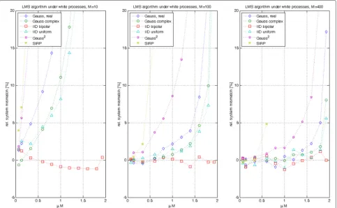
Experiment 1: In the first set of experiments, the white processes with properties in Table 2 were the driving source. The outcome of such experiments provides a vali-dation to the predicted steady-state behavior. For the long filter, (58) simplifies to
MS= μ M
2−μMm(f2,2), (65)
while (42) for the arbitrary LMS algorithm simplifies to the same expression with m(x2,2) replacingm(f2,2). This is in agreement with (76) (see Appendix 2) as for large fil-ter orderM; both terms become identical. Such simplified formula is often applied in practice. As we expect differ-ences only if the step-size is large, the precision of the formula is investigated in this experiment.
Figure 1 presents the relative errors 1− M¯S
MS obtained, in
percentage terms when applying (65). The results are as follows:
1. In all distributions, the errors obtained for small step-sizes are very small, confirming our theoretical predictions.
2. The larger the filter lengthM, the smaller the errors. This is expected as formula (65) was not only derived for long filters but also for small step-sizes, which are unavoidable for large filter lengths.
3. Only in the case ofM=10, for which a significant
γx=1is expected, the errors are moderate to large compared to the other cases.
Fig. 1Relative system mismatch(MS− ¯MS)/MSin percent based on simplified formula for white driving processes with different filter lengths
(M= {10, 100, 400})
results in the figure clearly show the impact of our asymptotic equivalence assumption, as the mismatch decreases with smaller step-sizes (which is a
consequence of higher filter orderM ).
5. Even for the SIRPs, our prediction is excellent. Note, however, that this depends very much on how an SIRP is modeled. AK0SIRP is generated by a product process of a Gaussian process with a random variable that is itself Gaussian distributed. If this RV, serving as the standard deviation of the process and defining its variance, is kept constant for each simulation run, the ensemble average will not converge. As the RV can take on arbitrarily large values (high energy driving process), the adaptation process can become extremely slow for some runs due to its fixed step-size. But even worse, as there is a finite probability that the variance of this process is below any bound, a fixed step-size is then too large for these runs to become stable. Such SIRP processes are only possible in the context of the normalized LMS (NLMS) algorithm. The situation is considerably better if the RV that defines the variance of the random process is itself generated by a random process, producing a slight change at every time instant so as to slowly modify the signal’s variance
over time, as is commonly done to resemble speech signals with their slowly changing variance. Note that for SIRPs,m(x2,2)=3, restricting the step-size range considerably (the stability bound is roughly at
μlimM=2/3).
The step-size range in Fig. 1 is limited to μ =
{1,. . ., 29} ×1/[ 15M]. The problem with higher step-size values is that the fluctuations become larger and thus sig-nificantly longer averaging is required (see also [32] for explanations of this effect), this not being feasible. In par-ticular for short filters (M=10), the convergence bounds are alternated byγx and thus the classical bound (3) is still too high. This can be observed very clearly for the IID Gauss2process, which leads to extremely high errors, when operating in close vicinity to the stability bound.
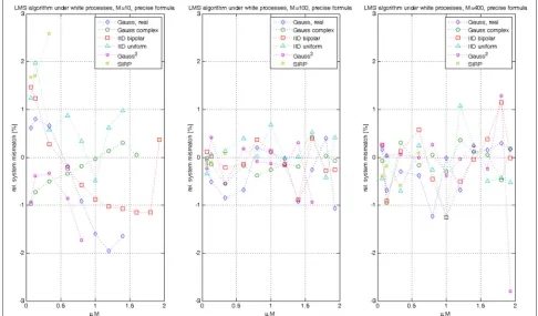
Experiment 2: We repeat the previous experiment, but we compare the results with the much more precise bound derived from (42) for a white driving process (real-valued):
MS= μMσ 2
v
2−μm(x2,2)(2+γxM)
= μMσv2
2−μm(x2,2)
M−1+ m(x4) m(x2,2)
.
In case the process is complex-valued, the bound (44) sim-plifies to a similar expression as (66); just the termM−1 in the denominator is to be replaced byM−2.
Figure 2 depicts the results. The major difference now is that the precision becomes much higher even for those processes that are far away from Gaussian (for exam-ple Gauss2). No matter what distribution or length of the filter, the error obtained remains below roughly 1 % as long as the step-size does not reach the stability bound.
We compare now our observations for the predicted sta-bility bound (48), which reads in our case for real-valued processes:
0< μ≤ 2
m(x2,2)
M−1+ m(x4) m(x2,2)
. (67)
We recognize that for large M, we find μlimM = 2/m(x2,2), thus 2 in general and 2/3 for SIRPs. For small val-ues ofM, the situation is different and we obtainμlimM=
{10/6 = 1.66, 20/11 = 1.81, 2, 20/10.8 = 1.85, 10/9 = 1.11, 5/9 = 0.55} for our six processes, an excellent agreement when compared to the left hand side of Fig. 2.
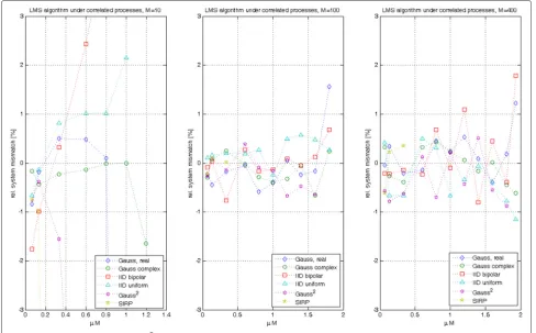
Experiment 3: In a last set of experiments, the previous simulation runs from Experiments 1 and 2 were repeated
for correlated driving processes. We applied a linear filter with impulse response
ak =0.6×0.8k; k=0, 1,. . . (68)
on the six driving processes of the previous experi-ment. The so-obtained AR(1) process with unit gain exhibits a relatively high correlation as it is com-mon in speech processes. If as in this case, the filter A(q−1) = 1−0.80.6q−1 becomes very long (P → ∞), the
largest eigenvalue becomes small compared to tr[Ruu]. Thus, the convergence bound for μbecomes practically 2/
m(f2,2)tr[Ruu] , which agrees well with our simula-tion results. Note that such bound can be much larger as well as much smaller than the classic bound in (3), depending on the value of m(f2,2). In Fig. 3, we compare our simulation results with the predicted values from (42) and (44), for real- and complex-valued processes, respectively. As before, we find excellent agreement in the order of 1 % error. For a small filter length M = 10, the largest eigenvalue becomesλmax = 5.5 and the predicted stability bounds are reduced from μlimM =
{1.66, 1.81, 2, 1.85, 1.11, 0.55} of the white driving pro-cesses toμlimM= {0.95, 1.29, 1.05, 1.01, 0.74, 0.31}which is well reflected in the simulation results. For larger filters, the stability bound moves towards μlimM → 2 (2/3 for
Fig. 2Relative system mismatch(MS− ¯MS)/MSin percent based on precise formula for white driving processes with different filter lengths
Fig. 3Relative system mismatch(MS− ¯MS)/MSin percent of correlated AR(1) driving processes
SIRP) for all processes, independent of the correlation. For M=400, the largest eigenvalue has only slightly increased toλmax=8.9 and thus has little influence on the stability bound.
We finally are interested in the fluctuations of the vari-ous runs (see [32]), defined in (64), which are evaluated at steady state now:
ρ= lim
k→∞ρk =klim→∞
!
var" ˜w||2k#
E ˜w||2k . (69)
As expected, the fluctuations, depicted in Fig. 4, increase considerably only for step-sizes close to the stability bound. For the very long filter, such bound was correctly predicted in (61), independent of pdf and correlation.
6 Conclusions
In this contribution, a stochastic analysis of second-order moments in terms of the parameter error covariance matrix has been shown for the LMS algorithm under the large class of linearly filtered random driving pro-cesses. While results were previously only known for a small number of statistics, this contribution deals with the large class of linearly filtered white processes with arbitrary statistics. Particularly interesting is the fact that
Fig. 4Fluctuationsρas a function ofμMfor three different filter lengths (M= {10, 100, 400}) of correlated AR(1) driving processes
be known, but note that also for classic results, the second-order moments, i.e., the autocorrelation matrix, needed to be known a priori (or estimated). Bringing in more parameters is the price of having a more general form of theory.
Endnotes
1Naturally, the basic LMS algorithm requires
modification to apply it successfully in various applications; we simply refer here to the entire family with similar algorithmic structure whose core elements are the LMS algorithm. Worth mentioning is in any case the normalized version NLMS of the LMS algorithm that ensures independence of the input’s signal power. Such small modification alone, however, already complicates the analysis substantially [11, 33]. Even for very long filters, non-Gaussian excitation such as speech signals can lead to severe problems [34] if no normalization is applied.
2The termswhiteanddecorrelatedwill henceforth be
used interchangeably.
3Note that the requirement of having statistically
independent regression vectors is actually far too strong as we only need to ensure thatEukukT(w−wk)
(w−wk)TukukT
=EukukTKkukukT
. One could also call itindependence approximationand just require this property.
4The procedure for obtaining such result is the same as
explained in the following paragraph forK , only much simpler, as the trace terms do not appear.
Appendix
Appendix 1: decomposition of symmetric matrices
A problem in the derivation of the LMS behavior is that the covariance matrices as they appear for the param-eter error vector Kk = E
(w−wk)(w−wk)T
are in general not in the modal space of the driving pro-cessuk =
uk,uk−1,. . .,uk−M+1
T
with autocorrelation matrixRuu=E
ukukT
=QuQTthus
Kk =b0I+b1Ruu+b2R2uu+. . . (70)
Since the derivation of the LMS algorithm only requires that the trace of such matrices be known, it is sufficient to analyze only the algorithm’s impact on the parameter error vector with respect toRuu. It is therefore proposed to decompose a given matrix Kinto a first part, i.e., in the modal space of the autocorrelation matrixRuuof the driving process uk and a second part in its orthogonal
complement space, i.e.,
Here,P(Ruu)denotes a polynomial inRuu. Note that due to the Cayley-Hamilton theorem, an exponent larger than M−1, withMdenoting the system order, is not required [28].
Lemma 1.Any symmetric matrixKcan be decomposed
into a part from the subspace of a given modal spaceRu= span"I,Ruu,Ruu2 ,. . .,RMuu−1
#
and its orthogonal comple-ment subspaceR⊥u for which trK⊥Rluu=0for any value of l=0, 1, 2,. . ..
Proof.The optimal set of coefficients for approximating the symmetric matrixKis found by
min
which is a simple quadratic problem with linear solution:
⎡ to the orthogonality property of the least squares solution, it is found that
As a further consequence terms of the form trRmuuK⊥Rluu = 0, and thusRmuuK⊥Rluu ∈ R⊥u, and any polynomialP(Ruu) ∈ Ru. Note that it is straightforward to extend the results to Hermitian matrices that occur for complex-valued processes.
Appendix 2: relation to higher order moments
Here, the second- and fourth-order moments are consid-ered once a random process is Fourier-transformed by a unitary matrixF. Assume a random processxk with the
properties (9)–(17). Take M consecutive values of such process, build a vector xk, and convert it to its Fourier
transform byfk =Fxk.
It is straightforward to show that the processfk is zero
mean ifxkis zero mean and, due to the unitary property
ofF, it is found thatm(f2)=E[|fk|2]=1 as long asm(x2)= E[|xk|2]=1.
For the fourth-order moments, the expression ExkxkTghHxkxkT
is considered, where g and h are
simply two different rows ofF, thusgHh=gTh= 0 and
From here, the following can be computed:
m(f2,2)=E
The latter relation is simply due to the fact that each element of the DFT matrix F is a rotation scaled by 1/√M. ForM→ ∞, it is concluded thatmf(2,2) = m(x2,2). The result would not change ifxk ∈ CI. It is in fact this
equivalence that convinced us to use m(2,2) rather than m(4)in our formulations. Note also that the termγxfrom (25) shows up here again. It is thus the correction term for the joint fourth-order moment that only has an impact on small filter dimensions.
Similarly, for the fourth-order moment, select g = h
and obtain m(f4) ≤ 2m(x2,2) +
are thus preserved under DFT for very long filters. Fur-thermore, regardless of the input process, after DFT of the long sequence, it is always found thatm(f4) =2m(f2,2), which significantly simplifies subsequent analysis.
Additional file
Additional file 1: MATLAB code.The MATLAB code for the experiments is publicly available at https://www.nt.tuwien.ac.at/downloads/. (ZIP 60 kb)
Competing interests
The author declares that he has no competing interests.
Authors’ information
networks and active noise control. From October 1995 until August 2001, he was a member of Technical Staff in the Wireless Technology Research Department of Bell-Labs at Crawford Hill, NJ, where he worked on various topics related to adaptive equalization and rapid implementation for IS-136, 802.11 and UMTS. Since October 2001, he is a full professor for Digital Signal Processing in Mobile Communications at the Vienna University of Technology where he founded the Christian-Doppler Laboratory for Design Methodology of Signal Processing Algorithms in 2002 at the Institute of Communications and RF Engineering. He served as Dean from 2005 to 2007 and from 2016-2017. He was an associate editor of IEEE Transactions on Signal Processing from 2002 to 2005, is currently an associate editor of JASP EURASIP Journal of Advances in Signal Processing, JES EURASIP Journal on Embedded Systems. He is an elected AdCom member of EURASIP since 2004 and serving as the president of EURASIP from 2009 to 2010. He authored and co-authored more than 500 papers and patents on adaptive filtering, wireless communications, and rapid prototyping, as well as automatic design methods. He is a Fellow of the IEEE.
Received: 3 June 2015 Accepted: 25 November 2015
References
1. B Widrow, ME Hoff Jr, inIRE WESCON Conv. Rec. Adaptive switching circuits, vol. Part 4, (1960), pp. 96–104
2. E Hänsler, G Schmidt,Acoustic Echo and Noise Control. (John Wiley & Sons, Chichester, New York, Brisabne, Toronto, Singapore, 2004)
3. M Rupp, Convergence properties of adaptive equalizer algorithms. IEEE Trans. Signal Process.59(6), 2562–2574 (2011)
4. AH Sayed, M Rupp, inProc. SPIE 1995. A time-domain feedback analysis of adaptive gradient algorithms via the small gain theorem, (San Diego, USA, 1995), pp. 458–469
5. M Rupp, AH Sayed, A time-domain feedback analysis of filtered-error adaptive gradient algorithms. IEEE Trans. Signal Process.44(6), 1428–1439 (1996). doi:10.1109/78.506609
6. AH Sayed, M Rupp, Error-energy bounds for adaptive gradient algorithms. IEEE Trans. Signal Process.44(8), 1982–1989 (1996). doi:10.1109/78.533719 7. AH Sayed, M Rupp, inThe DSP Handbook. Robustness issues in adaptive
filtering (CRC Press, Florida, 1998)
8. G Ungerboeck, Theory on the speed of convergence in adaptive equalizers for digital communication. IBM J. Res. Dev.16(6), 546–555 (1972)
9. LL Horowitz, KD Senne, Performance advantage of complex LMS for controlling narrow-band adaptive arrays. IEEE Trans. Signal Process.29, 722–736 (1981)
10. A Feuer, E Weinstein, Convergence analysis of LMS filters with uncorrelated Gaussian data. IEEE Trans. Acoust. Speech Signal Process. ASSP–33(1), 222–230 (1985)
11. M Rupp, The behavior of LMS and NLMS algorithms in the presence of spherically invariant processes. IEEE Trans. Signal Process.41(3), 1149–1160 (1993)
12. M Rupp, Adaptive filters: Stable but not convergent. EURASIP J. Adv. Signal Process. (2015)
13. S Haykin,Adaptive Filter Theory. (Prentice–Hall, Inf. and System Sciences Series, Englewood Cliffs, NJ, 1986)
14. JE Mazo, On the independence theory of equalizer convergence. Bell Syst. Technical J.58(5), 963–993 (1979)
15. R Nitzberg, Normalized LMS algorithm degradation due to estimation noise. IEEE Trans. Aerospace Electron. Syst.AES-22(6), 740–750 (1986). doi:10.1109/TAES.1986.310809
16. O Macchi,Adaptive Processing. (John Wiley & Sons, Chichester, New York, Brisabne, Toronto, Singapore, 1995)
17. V Solo, X Kong,Adaptive Signal Processing Algorithms. Prentice-Hall information and system sciences series. (Prentice-Hall, Englewood Cliffs (NJ), USA, 1995)
18. H-J Butterweck, inInternational Conference on Acoustics, Speech, and Signal Processing (ICASSP-95). A steady-state analysis of the LMS adaptive algorithm without use of the independence assumption, vol. 2, (1995), pp. 1404–1407. doi:10.1109/ICASSP.1995.480504
19. SC Douglas, TH-Y Meng, inProc. IEEE International Conf. on Acoustics, Speech, and Signal Processing. Exact expectation analysis of the LMS adaptive filter without the independence assumption, (San Francisco, CA, 1992), pp. 61–64
20. SC Douglas, W Pan, Exact expectation analysis of the LMS adaptive filter. IEEE Trans. Signal Process.43(12), 2863–2871 (1995). doi:10.1109/ 78.476430
21. TY Al-Naffouri, AH Sayed, Transient analysis of data-normalized adaptive filters. IEEE Trans. Signal Process.51(3), 639–652 (2003). doi:10.1109/TSP. 2002.808106
22. AH Sayed,Fundamentals of Adaptive Filtering. (John Wiley & Sons, Inc., Hoboken (NJ), USA, 2003)
23. H-J Butterweck, Iterative analysis of the steady-state weight fluctuations in LMS-type adaptive filters. IEEE Trans. Signal Process.47(9), 2558–2561 (1999)
24. H-J Butterweck, A wave theory of long adaptive filters. IEEE Trans. Circ. Syst. I: Fundamental Theory Appl.48(6), 739–747 (2001)
25. H-J Butterweck, Steady-state analysis of the long LMS adaptive filter. Signal Process. Elsevier.91(4), 690–701 (2011). doi:10.1016/j.sigpro.2010.07.015 26. SJM de Almeida, JCM Bermudez, NJ Bershad, A stochastic model for a
pseudo affine projection algorithm. IEEE Trans. Signal Process.57, 117–118 (2009)
27. HIK Rao, B Farhang-Boroujeny, Analysis of the stereophonic LMS/Newton algorithm and impact of signal nonlinearity on its convergence behavior. IEEE Trans. Signal Process.58(12), 6080–6092 (2010). doi:10.1109/TSP. 2010.2074198
28. M Rupp, H-J Butterweck, inProc. of the 37th Asilomar Conference. Overcoming the independence assumption in LMS filtering, vol. 1, (2003), pp. 607–611
29. DG Manolakis, VK Ingle, SM Kogon,Statistical and Adaptive Signal Processing. (Artech House, Boston, London, 2005)
30. WA Gardner, Learning characteristics of stochastic gradient descent algorithms: a general study, analysis and critique. Signal Process.6(2), 113–133 (1984)
31. RM Gray,Toeplitz and Circulant Matrices: A Review. Foundations and Trends in Communications and Information Theory, vol. 2. (Now publisher, Delft, 2006), pp. 155–239
32. VH Nascimento, AH Sayed, On the learning mechanism of adaptive filters. IEEE Trans. Signal Process.48(6), 1609–1625 (2000). doi:10.1109/78.845919 33. NJ Bershad, Analysis of the normalized LMS algorithm with Gaussian
inputs. IEEE Trans. Acoust. Speech Signal Process.34(4), 793–806 (1986) 34. M Rupp, Bursting in the LMS algorithm. IEEE Trans. Signal Process.43(10),
2414–2417 (1995)
Submit your manuscript to a
journal and benefi t from:
7Convenient online submission 7Rigorous peer review
7Immediate publication on acceptance 7Open access: articles freely available online 7High visibility within the fi eld
7Retaining the copyright to your article