A comparison of a model using the FORMOSAT-3/COSMIC data
with the IRI model
Yoshihiro Kakinami1∗, Jann-Yenq Liu1,2, and Lung-Chih Tsai2
1Institute of Space Science, National Central University, No. 300 Jhongda Rd. Jhongli, Taoyuan 32001, Taiwan
2Center for Space and Remote Sensing Research, National Central University, No. 300 Jhongda Rd. Jhongli, Taoyuan 32001, Taiwan
(Received August 18, 2010; Revised January 4, 2011; Accepted October 8, 2011; Online published July 27, 2012)
In this study, an empirical model constructed using data of FORMOSAT3/COSMIC (F3/C) from 29 June, 2006, to 17 October, 2009, retrieves altitude profiles of electron density (Ne). The model derives global Ne
profiles from 150 to 590 km altitude as functions of the solar EUV flux, day of year, local time and location under geomagnetically quiet conditions (Kp <4). Neprofiles derived by the model are further compared with those
of the International Reference Ionosphere (IRI). Results show that the F2 peak altitudehmF2and the electron
densityNmF2, as well as the electron density above, derived by the model are lower than those of the IRI model.
The F3/C model reproduces observations of F3/C well at 410-km altitude while the IRI model overestimates them. The overestimation of the IRI model becomes large with decrease of EUV flux. It is found that the topside vertical scale height of the F3/C model shows high values not only magnetic dip equator but also middle latitude. The results differ significantly from those of IRI, but agree with those observed by topside sounders, Alouette and ISIS satellites.
Key words:IRI, electron density, topside ionosphere, empirical model, FORMOSAT-3/COSMIC, vertical scale
height.
1.
Introduction
The International Reference Ionosphere (IRI) has been developed since 1978 (Rawer et al., 1978) and is estab-lished as the most standard and reliable ionospheric empiri-cal model. Since a large amount of ionosonde data has been used, IRI derives a relatively accurate electron density (Ne)
profile below the F2 peak. However, the IRI model might
still have some shortcomings in the topside ionosphere, be-cause very limited satellite data are included. Bilitza (2004) and Bilitza et al. (2006) based on Alouette/ISIS topside sounder observations reported that the IRI model overesti-matesNeabove theF2peak height. Furthermore, Kakinami
et al.(2008) found an in-situ Neobservation at a 600-km
altitude with the Hinotori satellite which differed from the IRI Ne. This shortcoming also results in a difference
be-tween the Total Electron Content (TEC) reproduction and real observations, because the TEC is calculated using an integration of the Ne profile. Meanwhile, the IRI model
overestimates the TEC in the equatorial region (Bilitza and Williamson, 2000) during high solar activity, while the IRI model overestimates and underestimates the TEC over Tai-wan (24◦N 120◦E) during low and high solar activity, re-spectively (Kakinamiet al., 2009).
∗Now at Institute of Seismology and Volcanology, Hokkaido
Univer-sity, Kita 10 Nishi 8, Kita-ku, Sapporo 060-0810, Japan.
Copyright cThe Society of Geomagnetism and Earth, Planetary and Space Sci-ences (SGEPSS); The Seismological Society of Japan; The Volcanological Society of Japan; The Geodetic Society of Japan; The Japanese Society for Planetary Sci-ences; TERRAPUB.
doi:10.5047/eps.2011.10.017
Six FORMOSAT-3/COSMIC (F3/C) micro satellites which constituted a global positioning system (GPS) oc-cultation experiment (GOX) payload were launched on 14 April, 2006, and put into a low Earth orbit of 800-km al-titude with a 72◦inclination. An average of 1800 electron density profiles was obtained in a day globally. Leiet al.
(2007) reported that Ne profiles measured with F3/C are
consistent with NmF2 andhmF2 obtained with incoherent
scatter radars at Millstone Hill and Jicamarca. AnNe
pro-file obtained using GOX has an advantage in its coverage of observations, compared with the peak density and peak altitude of the ionosphere obtained with ground-based ob-servations, because it was able to cover ocean and desert areas, where there are usually no receivers. Taking advan-tage of this feature, we have constructed an empirical model of theNeprofile measured with F3/C, which reproduces the
Neprofile globally. In this paper, we describe the
method-ology in constructing the model and compare the empirical model based on F3/C observations with the IRI model.
2.
Methodology of the Construction of an
Empir-ical Model
The methodology of constructing an empirical model based on F3/C data is described in this section. Hence-forth, the empirical model based on Ne profiles obtained
by F3/C is referred to as the F3/C model. The F3/C model reproduces Ne as functions of the solar EUV flux,
day of year (DOY), local time (LT), altitude and loca-tion. A similar methodology has been applied to em-pirical models of transition height (Marinov et al., 2004; Kutiev and Marinov, 2007), vertical scale height in the
symmetry, the errors mainly appear below 250 km around the equatorial ionization anomaly region (Liuet al., 2010), which leads to a negative value of the Neprofile in some
cases. Therefore, observed Neprofiles showing a negative
value are not used in the model construction. At first, the empirical model which has functions of EUV, DOY and LT is constructed in each 3-dimensional bin whose size is 30◦ in longitude, 18◦in latitude and 20 km (40 km) altitude be-tween 150 and 390 (390 and 590) km altitude with steps of 10◦ in longitude and 6◦ in latitude. It is assumed that the solar flux variation of log10(Ne)is proportional to the
EUV flux, while the DOY and LT variation of log10(Ne)
are derived using a combination of trigonometric functions of wavenumbers 1–3 and 1–4, respectively. The modeled functions are calculated for each bin. The functions for F, DOY and LT are defined as follows:
f(EUV)=a1+a2EUV, (1)
wherea,b,care coefficients for fitting. DOY is normalized by the length of the year. The function reproducingNe is
assumed to be the product of these 3 functions. Then we can obtain: coefficients α, more than 126 data are required. The α can be obtained by solving the following normal-equation
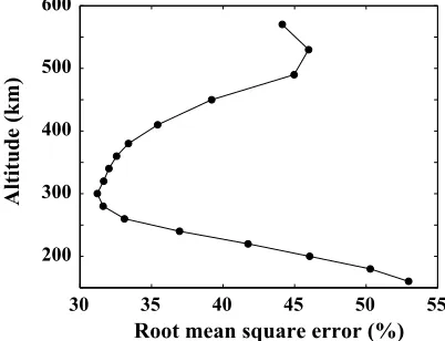
Fig. 2. Variation of root mean square error of the F3/C model with altitude.
matrix:
Theαare calculated in each 3-dimensional bin. Finally, the modeled Ne is obtained by linearly interpolating
be-tween the bins.
3.
Results and Discussion
In order to estimate the accuracy of the F3/C model, the root-mean-square error (RMS) is calculated as follows,
RMS=
with F3/C, and theNederived by the F3/C model,
Fig. 3. Comparison of peak electron density derived by the F3/C model and the IRI model with ionosonde observations at 1200 LT at Millstone Hill (left) and Darwin (right) from 29 June, 2006, to 17 October, 2009. Red and blue dots indicate the F3/C and the IRI model results.
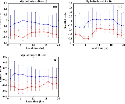
Fig. 4. Local time variation of the residual ratios for the F3/C (blue) and IRI (red) models in (a) dip latitude= −30∼ −10, (b) dip latitude= −10∼10 and (c) dip latitude=10∼30. Dots and error bars denote median and quartiles.
value at 300 km. The RMS increases with increasing al-titude over 300 km and reaches about 45% around 500 km. Below 250 km, the estimation error of theNeprofile is very
large due to the fundamental issue of the Abel inversion (Liu et al., 2010), and the data used in the construction have inherent errors. Such errors might produce a high dis-persion and show high RMS. On the other hand, since a similar high variability is seen in the Ne model using the
HINOTORI data at 600 km (Kakinami et al., 2008), the dispersion ofNemight be high above 400 km.
The peak Necalculated with the F3/C model are
median and quartiles.
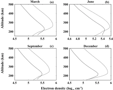
Fig. 6. Electron density profiles derived by the F3/C (solid line) and IRI models (dashed line) at 42.5◦N 288.5◦E at 1200 LT in March (a), June (b), September (c) and December (d). Intensities of EUV applied to calculations are 1.99, 1.99, 1.84 and 2.20×10¹¹photon/cm2sec, which are the actual conditions of solar flux in each month of 2007.
results with IRI match the observations at Millstone Hill, while those with the F3/C model overestimate the observa-tions. Meanwhile, both models overestimate at Darwin in many cases. This result indicates that the reproduction of peak density by the IRI also has shortcomings at some lo-cations.
In order to compare the observed Ne using F3/C with
the F3/C and IRI model, residual ratios, (oi −mi)/mi,
whereoiandmi denote the observedNeat 410 km and the
modeled Neat 410 km, are calculated. Figure 4 displays
the local time variation of the residual ratios for the F3/C and IRI models. Though the F3/C model slightly
overes-timates the observations by 10–20% during night time in all latitudes, the F3/C model agrees with the observations on the whole. However, the IRI model always overesti-mates observations by 40–60% at all local times and lati-tudes. Figure 5 shows the solar flux variation of the resid-ual ratios for the F3/C and IRI models. The F3/C model shows a good agreement with the observations except for EUV > 24×1010 photon/cm2 sec. As shown in Fig. 1,
since the data number for EUV > 24×1010 photon/cm2
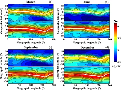
Fig. 7. Peak electron density maps derived by F3/C (top) and IRI model (bottom) at 1200 LT in March (a), June (b), September (c) and December (d). White curves indicate magnetic equator. Intensities of EUV applied to calculations are the same as Fig. 6.
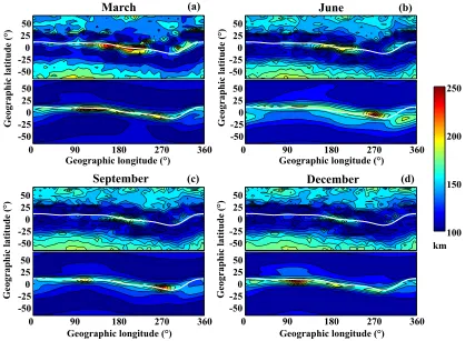
Fig. 9. Vertical scale height at 450 km derived by the F3/C model (top) and IRI model (bottom) at 1200 LT in March (a), June (b), September (c) and December (d). White curves indicate magnetic equator. Intensities of EUV applied in the calculations are the same as Fig. 6.
when EUV is low. The accuracy of the IRI model improves with an increase of EUV. This tendency of the IRI model to solar flux is similar to that of TEC over Taiwan (Kakinami
et al., 2009).
The altitude profile ofNederived by the F3/C and the IRI
models above Inamori Hall, Kagoshima University (42.5◦N 288.5◦E), where the IRI 2009 workshop was held, are shown in Fig. 6. TheNederived by the IRI model is higher
than that of the F3/C model at, and above the peak height in all seasons as shown in Figs. 4 and 5. In addition, the peak altitudehmF2derived by the IRI model is higher than that
of the F3/C model in all seasons. The vertical scale height (VSH) of the IRI model, which is defined as−dh/d(lnNe)
(Kutievet al., 2006), is slightly lower than that of the F3/C model in June. The Ne derived by IRI is lower than that
of the F3/C model in the lower ionosphere in all seasons except December.
Figure 7 shows the seasonal variation of peakNe(NmF2)
at 1200 LT derived by the F3/C (top panel) and the IRI (bottom panel) models. The maximum ofNmF2is located
beside the magnetic equator for both models. NmF2
de-rived by IRI is higher than that of the F3/C model in all seasons. A longitudinal structure of NmF2 exists in both
models. Small patch-like maxima of NmF2 appear in the
F3/C model, while wide-longitude-range maxima ofNmF2
appear in IRI in March (Fig. 7(a)). A four-peak (2-peak) longitudinal structure is detected in the F3/C (IRI) model in June. The IRI model shows a clear 2-peak longitudinal structure in September. On the other hand, the F3/C model displays a 2-peak or more small-scale longitudinal structure
in September. A four or three-peak structure appears in both models in December.
The seasonal variation of Ne at 450 km derived by the
F3/C and IRI models are shown in Fig. 8. TheNederived
by the IRI model is generally higher than that of the F3/C model around the magnetic equator. In contrast to theNmF2
shown in Fig. 7, a large-scale longitudinal structure, which is similarly reported by many scientists (e.g. Sagawaet al., 2005; Immelet al., 2006; Lin et al., 2007; Kakinami et al., 2011), is clearly seen around the magnetic equator in the F3/C model. According to Kakinami et al. (2011), the 4-peak structure of Ne at 660 km observed with the
DEMETER satellite is the most pronounced in September while a 3-peak structure appears in March and December. Though the IRI model also shows a longitudinal structure, the longitudinal structure retrieved with the F3/C model is more pronounced than that of the IRI and its seasonal variation agrees with previous studies.
Seasonal variations of VSH at 450 km derived by the F3/C and IRI models are shown in Fig. 9. The IRI model shows a maxima of VSH along the magnetic equator with a 10◦ latitude width while the F3/C model only displays a small maxima of VSH around 140–240◦E and 300◦E near the magnetic equator. In the F3/C model, maxima of VSH around 140–240◦E near the magnetic equator are always significant in all seasons, which show a maximum value in March. However, a maximum of VSH around 300◦E is only significant in March. The longitudinal structure seen in the VSH derived by the F3/C model differs from those of Ne
derived by the IRI model appear around the magnetic equa-tor. The location of each peak roughly corresponds to the locations of the maximum ofNeshown in Fig. 8. A
signif-icant difference in the VSH between the F3/C and the IRI models appears in the middle latitude. The VSH derived by the IRI model only shows a maximum around the magnetic equator, a sharp drop away from the magnetic equator and is almost constant in low and middle latitudes. Meanwhile, VSH derived by the F3/C model shows maxima (minima) around magnetic equator (beside geomagnetic equator) and increases with increasing latitude in low and middle lati-tudes. Similar VSH results are observed not only in F3/C data (Liuet al., 2008) but also by the topside sounder on-board the Alouette and ISIS satellites (Kutiev and Marinov, 2007). Especially, VHS derived by the F3/C model higher than 50◦S is higher than the magnetic equator in September and December.
4.
Summary
We have constructed an empirical model based on Ne
profiles observed with F3/C under geomagnetically quiet conditions (Kp < 4). The F3/C model derives globalNe
profiles between altitudes of 150 and 590 km as functions of the solar EUV flux, day of year, local time and loca-tion. TheNeabove theF2peak, and the F2 peak altitude,
derived by the F3/C model is lower than those derived by the IRI. The F3/C model reproduces a longitudinal struc-ture better than the IRI model. The F3/C model also de-rives VSH which show good agreement with measurements obtained from topside sounders onboard the Alouette and ISIS satellites. Since the F3/C model has a big advantage of greater data coverage, it helps us to understand a variety of upper ionospheric phenomenon. As a result, the F3/C model contributes an improvement over the IRI model.
Acknowledgments. This work was partially supported by the Earth Observation Research Center, Japan Aerospace Exploration Agency (Y. K.) and the National Science Council project NSC 98-2116-M-008-006-MY3 grant of the National Central University (Y. K. and J. Y. L.).
References
Bilitza, D., A correction for the IRI topside electron density model based on Alouette/ISIS topside sounder data,Adv. Space Res.,33, 838–843, 2004.
Bilitza, D. and R. Williamson, Towards a better representation of the IRI topside based on ISIS and Alouette data,Adv. Space Res.,25(1), 149– 152, 2000.
Bilitza, D., B. W. Reinsch, S. Radicella, S. Pulinets, T. Gulyaeva, and L. Triskova, Improvements of the international reference ionosphere
model for the topside electron density profile,Radio Sci.,41, RS5S15, doi:10.1029/2005RS003370, 2006.
Immel, T. J., E. Sagawa, S. L. England, S. B. Henderson, M. E. Hagan, S. B. Mende, H. U. Frey, C. M. Swenson, and L. J. Paxton, Control of equatorial ionospheric morphology by atmospheric tides,Geophys. Res. Lett.,33, L15108, doi:10.1029/2006GL026161, 2006.
Judge, D. L., D. R. McMullin, S. Ogawa, D. Hovestadt, B. Klecker, M. Hilchenbach, L. R. Canfield, R. E. Vest, R. Watts, C. Tarrio, M. Kuhne, and P. Wurz, First solar EUV irradiances obtained from SOHO by the CELIAS/SEM,Sol. Phys.,177, 161–173, 1998.
Kakinami, Y., S. Watanabe, and K.-I. Oyama, An empirical model of electron density in low latitude at 600 km obtained by Hinotori satellite,
Adv. Space Res.,41, 1494–1498, doi:10.1016/j.asr.2007.09.031, 2008. Kakinami, Y., C. H. Chen, J. Y. Liu, K.-I. Oyama, W. H. Yang, and S. Abe,
Empirical models of Total Electron Content based on functional fitting over Taiwan during geomagnetic quiet condition,Ann. Geophys.,27, 3321–3333, 2009.
Kakinami, Y., C. H. Lin, J. Y. Liu, M. Kamogawa, S. Watanabe, and M. Parrot, Daytime longitudinal structure of electron density and tempera-ture in the topside ionosphere observed by the Hinotori and DEMETER satellites,J. Geophys. Res., doi:10.1029/2010JA015632, 2011. Kutiev, I. and P. Marinov, Topside sounder model of scale height and
transition height characteristics of the ionosphere,Adv. Space Res.,39, 759–766, 2007.
Kutiev, I., P. Marinov, and S. Watanabe, Model of topside ionosphere scale height based on topside sounder data,Adv. Space Res.,37, 943–950, 2006.
Lei, J., S. Syndergaard, A. G. Burns, S. C. Solomon, W. Wang, Z. Zeng, R. G. Roble, Q. Wu, Y.-H. Kuo, J. M. Holt, S.-R. Zhang, D. L. Hysell, F. S. Rodrigues, and C. H. Lin, Comparison of COS-MIC ionospheric measurements with ground-based observations and model predictions: Preliminary results,J. Geophys. Res.,112, A07308, doi:10.1029/2006JA012240, 2007.
Lin, C. H., W. Wang, M. E. Hagan, C. C. Hsiao, T. J. Immel, M. L. Hsu, J. Y. Liu, L. J. Paxton, T. W. Fang, and C. H. Liu, Plausible effect of atmo-spheric tides on the equatorial ionosphere observed by the FORMOSAT-3/COSMIC: Three-dimensional electron density structures,Geophys. Res. Lett.,34, L11112, doi:10.1029/2007GL029265, 2007.
Liu, L., M. He, W. Wan, and M.-L. Zhang, Topside ionospheric scale heights retrieved from Constellation Observing System for Meteorol-ogy, Ionosphere, and Climate radio occultation measurements,J. Geo-phys. Res.,113, A10304, doi:10.1029/2008JA013490, 2008.
Liu, J. Y., C. Y. Lin, C. H. Lin, H. F. Tsai, S. C. Solomon, Y. Y. Sun, I. T. Lee, W. S. Schreiner, and Y. H. Kuo, Artificial plasma cave in the low atitude ionosphere results from the radio occultation inver-sion of the FORMOSAT–3/COSMIC,J. Geophys. Res.,115, A07319, doi:10.1029/2009JA015079, 2010.
Marinov, P., I. Kutiev, and S. Watanabe, Empirical model of O+-H+ tran-sition height based on topside sounder data,Adv. Space Res.,34, 2021– 2025, 2004.
Rawer, K., D. Bilitza, and S. Ramakrishnan, Goals and status of interna-tional reference ionosphere,Rev. Geophys.,16, 177–181, 1978. Sagawa, E., T. J. Immel, H. U. Frey, and S. B. Mende,
Longitu-dinal structure of the equatorial anomaly in the nighttime iono-sphere observed by IMAGE/FUV, J. Geophys. Res., 110, A11302, doi:10.1029/2004JA010848, 2005.