A study of the storm event on October 21–22, 1999 by the MHD simulation

A study of the storm event on October 21–22, 1999 by the MHD simulation

K. S. Park and T. Ogino

Solar-Terrestrial Environment Laboratory, Nagoya University, Japan

(Received May 18, 2005; Revised January 14, 2006; Accepted January 16, 2006; Online published May 12, 2006)

We carried out a high resolution three-dimensional magnetohydrodynamic (MHD) simulation of the interac-tion between the solar wind and the Earth’s magnetosphere during a strong magnetic storm on October 21–22, 1999. The input to the simulation was from WIND solar wind observations. As the IMF is strongly south-ward (−20 nT to−30 nT) for 6 hours, the geomagnetic field lines in the dayside magnetopause are eroded to the geosynchronous orbit (GEO) region by reconnection. The associated magnetic flux is transferred from the dayside magnetosphere to the tail. The reconnection region still appears near GEO region on the dayside magne-topause, even though the IMFBzcomponent becomes small or northward, because of the influence of the strong IMFBy (30 nT). IMF lines can successively reconnect with the naked and large geomagnetic field line in the dayside flank regions. Thus, the cross polar cap potential is maintained to be large value and convection in the ionosphere is enhanced. The cross polar cap potential is governed by IMFByas well asBz (φ∼250 kV forBz

∼ −20 nT andφ∼300 kV for Bz∼ −30 nT), and it saturates during the strong southward IMF. A large energy flux enters the ionosphere at very low latitudes (50◦) and the inner edge of the plasma sheet becomes very close to the Earth (X = −3.2RE) for a strong magnetic storms. The open-closed boundary extends to 60◦latitudes on the nightside, 72◦on the dayside, 62◦on dawn, and 66◦on dusk. Enhanced energy flux appears at low latitudes (50◦) on the nightside in simulation. Moreover, the energy flux in the dusk region (19 MLT) appears down to 55◦ latitude in simulation, which is consistent with the low latitude boundary of the 0.02–20 keV particles detected by TED of the NOAA-15. A convective electric field, which is penetrating to the Earth-side of the NENL, is almost comparable to that of the solar wind. The present MHD simulation study give reasonable results even for extreme conditions and thereby its usefulness is demonstrated as a physical model for space weather studies.

Key words:A global MHD simulation, storm event study.

1.

Introduction

Early simulations of the interaction between the solar wind and the magnetosphere (Lyonet al., 1981; Brechtet al., 1981; Oginoet al., 1985; Walker et al., 1993) were applied to ideal cases in which the solar wind and the inter-planetary magnetic field (IMF) were constant.

In recent years, global MHD simulations have been used to model magnetospheric events by using actual solar wind observations as input. One of the first of these global MHD simulations was carried out by using the solar wind data for a 1-hour period on October 19, 1986 (Fedderet al., 1995). The solar wind velocity was high and almost constant with 660 km/s and IMFByandBzwere about−6 nT and−6 nT, respectively, in that event. They showed that closed field lines in the northern dusk region extended to higher lati-tudes due to the negative IMF By. In order to develop a Global Geospace Circulation Model (GGCM), MHD simu-lations were run for two time intervals on January 27, 1992 (1325–1715 UT and 1730–1930 UT) and were compared with observations (Raederet al., 1998; Lyons, 1998). The IMF was northward on average, with a largeBycomponent (By = −20 nT), and the dynamic pressure (Dp∼4 nPa) was about 2 to 3 times larger than normal. They found a

Copyright cThe Society of Geomagnetism and Earth, Planetary and Space

Sci-ences (SGEPSS); The Seismological Society of Japan; The Volcanological Society of Japan; The Geodetic Society of Japan; The Japanese Society for Planetary Sci-ences; TERRAPUB.

good qualitative agreement between the simulated potential patterns and those from the Assimilative Mapping of Iono-spheric Electrodynamics (AMIE) empirical model.

Raederet al.(2001) used a global model of Earth’s mag-netosphere and ionosphere to simulate the Geospace En-vironment Modeling (GEM) substorm challenge event on November 24, 1996, and the simulation of a substorm tim-ing was also studied by Slinkeret al.(2001), Lyonset al.

(2001) and Ashour-Abdalla et al.(2002b). In this event, northward IMF (∼ +5 nT) for∼80 min, followed by a sud-den rotation of the IMFsouthward (∼ −7 nT). The GEM substorm challenge event provided them with a unique opportunity to compare their model with observation and to assess its validity with respect to substorm dynamics. Ashour-Abdalla et al. (1999, 2002a) investigated a sub-storm during a very active period on December 22, 1996 and found a good agreement between the onset time of the substorm in their global MHD simulation and that inferred from Polar observation images. Le et al. (2001) used a simulation and data to investigate magnetospheric dynam-ics during an extended period of strongly northward IMF (20 nT) on April 11, 1997. They found that the location of the reconnection layer was in agreement with the Polar observations but the layer was much thinner than that pre-dicted by the MHD simulation. Global MHD simulations have been quite successful in reproducing overall magneto-spheric dynamics. They usually reproduce the time changes

that occur in the auroral ionosphere. However, there are a few simulations with a high spatial resolution to quantita-tively study the effects of a long time duration of strong southward IMF for magnetic storms. How much energy are transported from the solar wind through the magnetosphere into the ionosphere during such an extreme condition, and how is it transported? We also need to understand the mag-netospheric phenomena such as the dayside reconnection and potential saturation by the effects of large IMF Bzand

Bycomponent.

In this paper, we present the results of a strong mag-netic storm event study by using a three-dimensional global MHD model during which the IMF was strongly southward for a long time. We chose an event on October 22, 1999 during which strong auroral electrojet and ring current dis-turbances were observed. The dynamic pressure of solar wind varied from 1.8 to 51.8 nPa and the IMFBzwas about

−31 nT for three hours. The Kp index was 8- during this period and Dst reached −237 nT. In Section 2, we de-scribe the MHD simulation model. In Section 3, we ex-plain characteristic features of the events observations on October 22. Simulation results are presented in Section 4 and the chronology of simulated substorms are explained in Section 5. We discuss the results in comparison with obser-vations in Section 6. Finally, conclusions are summarized in Section 7.

2.

Simulation Model

2.1 Basic Equations

We have solved the normalized resistive MHD and Maxwell’s equations as an initial value problem by using a modified version of the Leap-Frog scheme. The basic MHD simulation model has been described in detail by Oginoet al.(1992). The normalized MHD equations are written as follows:

whereρis the plasma density,Vis the plasma flow velocity,

P is the plasma pressure,Bis the magnetic field,Bdis the dipole field of Earth,Jis the current density,g = −g0/ξ3

(ξ2 _{= x}2_+y2_+z2_,g

0 = 1.35×10−6 (9.8 m/s2)) is the force of gravity, μ∇2_{Vis the viscosity, andγ is the ratio} of specific heats; γ = 5/3. η = η0(T/T0)−3/2 is the resistivity, whereT = P/ρ is the temperature, and T0 is the ionospheric temperature. The model resistivityη0is set to 0.001 and the diffusion coefficient is D = Dp = μ0 =

μ/ρsw=0.001, whereρswis the solar wind plasma density. The magnetic Reynolds number is S = τ_η/τA = 100–2000 whereτ_η ≡ x2_/η,τ

A= x/VA, and xis the mesh size. The normalized quantities in the basic equations are the

radius of the Earth, RE =6.37×106 m, the Alfv´en transit magnetospheric coordinates. For this simulation the bound-aries are X0 =30 RE, X1 = −120 RE,Y0 =60 RE, and

−Z1 = Z0 = 60 RE. A mirror dipole field is applied in the solar wind at time t = 0 to take up the shape of the mag-netopause. Watanabe and Sato (1990) have shown that this initial condition helps assure that∇ ·B= 0 throughout the simulation box. The Earth is located at the origin of the sim-ulation box,r= (X,Y,Z)=(0 RE, 0RE, 0 RE) and the solar wind flows into the box in theX-direction through the upstream boundary at X = X0. The number of grid points is(nX,nY,nZ)=(500,200,400)with a uniform grid spac-ing of X =0.3 RE. The following boundary conditions are imposed for each physical quantity,φ =(ρ,V,P,B). At the upstream boundary for X = X0, we use 1 minute solar wind data acquired by the WIND satellite as input pa-rameters (ρ,Vx,P,By,Bz) of the simulation. The IMFBx component is not used to keep a layered structure of the IMF lines in the solar wind. The WIND parameters are sampled at different times so we used linear interpolation to calculate all of the parameters at the same time.

The simulation quantities are connected with the solar wind quantity at each proper time step (32 t) by introduc-tion of a smooth funcintroduc-tion, where t is a time step. The in-ternal quantity,φin, at the initial state in the ionosphere and the external quantity of the simulated parameter, φex, are connected at each time step by the introduction of a smooth function, f

φ= fφex+(1− f)φin,

where f ≡a0h2/(a0h2+1),a0=100,h =(ξ/ξa)2−1 for

ξ ≥ξa, andh =0 forξ < ξa. The smooth function damps out all perturbations near the ionosphere including parallel currents. Therefore the parallel currents do not close in the ionosphere, rather they partly close in the smoothing region above the ionospheric boundary. The internal ionospheric boundary conditions are set by forcing a static equilibrium atξa = 2.5 RE. We reduce radius of the internal bound-ary from our previous simulation to more accurately simu-late inner magnetospheric dynamics during strong magnetic storm events. The normalized MHD equations are solved as an initial value problem under the boundary conditions by using a modified version of the Leap-Frog method in or-der to obtain quasi steady state magnetospheric configura-tion. The simulation time step, t (=0.14 s), is given from the numerical stability condition of the differential scheme,

Vmax g

t

x < 1, whereVgmaxis the maximum group velocity in the simulation volume.

2.3 Magnetosphere-Ionosphere Relationship

there are two methods to treat magnetosphere-ionosphere coupling. In the first method, the field-aligned currents (FACs),J, are mapped from inner boundary of the magne-tosphere to the ionosphere along magnetic field lines. The equations giving the relationship between the parallel cur-rent and the electric potential are given in (6–8) whereφis the electric potential,is the ionospheric conductance ten-sor, andJis the parallel current density. Equations (6), (7), and (8) are used to calculate the velocity,V_⊥, and electric field,E_⊥, which are then mapped from the ionosphere back to the magnetosphere.

J= ∇ ·· ∇φ (6)

E⊥= −∇φ (7)

V_⊥= E⊥×B

B2 (8)

J_⊥=·E_⊥ (9)

If is only the Pedersen conductivity and a constant, we have

∇2_φ=J

−1. (10)

Then incompressibility condition is automatically satisfied as

∇ ×E_⊥=0

∇ ·V_⊥=0.

Equation (10) shows the relationship among J,, andφ.

φandV⊥are surely related to. Ifdouble for constant

J,φandV⊥should be half.can be fundamentally deter-mined by the ionospheric parameter such as the density, the temperature of the plasma, neutral gases, and the magnetic field.

In the second method, the magnetosphere and the iono-sphere coupling process is handled by a reversing the pro-cedure. Each velocity, V_⊥, or electric field, E_⊥ (E_⊥ = −V_⊥×B), is mapped directly from the inner boundary of the magnetosphere to the ionosphere along magnetic field lines, and then the parallel current density, J, is inversely mapped from the ionosphere to the magnetosphere to cal-culate a perturbation of the magnetic field as follows,

E_⊥= −V_⊥×B (11)

J⊥=·E⊥ (12)

J = −∇_⊥··E_⊥ (13)

IfE⊥ =−∇φis assumed, the ionospheric potential and the parallel current density are calculated by using the rela-tionship∇2_{φ=∇ ·(V}

⊥×B)andJ=∇ ·· ∇φ. If a magnetic flux function,ψ, is introduced in cylindrical coordinate for simplicity, the following relation is given;

B=Z× ∇ψ, (14)

whereZis the unit vector in Z-direction. It can be calcu-lated from the FACs, J, at the inner boundary of the mag-netosphere as follows

∇2_ψ=

J. (15)

Therefore, the magnetic field can be approximately ob-tained from Eq. (14).

In this case, incompressibility was not assumed in (11). Then the following conditions hold;

∇ ×E_⊥=0

∇ ·V_⊥=0,

in which the relationship ofE_⊥ = −∇φis never assumed. It is noted that the incompressibility condition is not re-quired in the ionosphere for the second method. In this sim-ulation, a constant Pedersen conductivity in the ionosphere is assumed to be 7 S, which is obtained from the condition that the potential peaks given by the two different methods are the same.

3.

Characteristic Features of October 21–22

Events

Figure 1 shows the auroral electrojet index (top panel) and the magnetic storm disturbances index, Dst, (bottom panel) for the October 21–22, 1999, storm. During this pe-riod, the AL index had a double minimum: the first min-imum of−1357 nT occurred at 0104 UT and the second minimum of −1992 nT was at 0431 UT. Dst reached a minimum value of−237 nT at 0600-0700 UT.

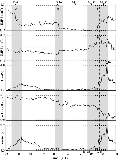
WIND observations of the solar wind and the IMF are shown in Fig. 2 for the period from 2300 UT on October 21 to 0800 UT on the next day. The time was shifted by 4∼6 min to account for the travel time from the WIND observation (located at X ∼ 29 RE) to the Earth. The Figure shows, from top to bottom, IMF Bz, By, dynamic pressure (Dp), velocity (Vx), and the number density. The IMF Bz was southward (−20 to −30 nT) for ∼6 hours. The IMF Bywas dawnward until 0540 UT, when it turned duskward, reaching ∼30 nT. There were two peaks in the solar wind dynamic pressure, the second peak reached

∼52 nPa at 0716 UT. ¿From these solar wind and the IMF variations, it was expected that the strong storm event could be generated by strong southward IMF for a long duration and by increased of the solar wind dynamic pressure.

4.

Simulation Results

Figure 3 shows the time evolution of the electric potential from the simulation, whereφ(+),φ(−), andφ(+)−φ(−) are the maximum, the minimum and cross polar cap poten-tial respectively, and shaded portions of A, B and C indicate the times highlighted in Fig. 2. A few minutes after the ar-rival of the southward (Bz∼−20 nT) from 2348 UT in the state of northward IMF, the cross polar cap potential de-creases once at 2359 UT by convection reversal and then increases by nearly 240 kV. It remains nearly constant un-til after the second decrease inBz(∼−30 nT) at 0316 UT. After that, it increases gradually to ∼300 kV. Lui et al.

AU, A L Indices [nT]

500

AU

AL

0

-500

-1000

-1500

-2000

23 24 01 02 03 04 05 06 07 08

0104/22

0431/22

Universal Time (Hours)

Dst Index [nT] 50

0

-50

-100

-150

-200

-250

0/21 12 0/22 12 0/23 12 0/24

06-07/22

Universal Time (Hours)

Fig. 1. Time variations of the AU, AL indices (top) and Dst index (bottom). The AL index had a minimum of−1992 nT at 0431 UT and the Dst index was a minimum of−237 nT at 0600-0700 UT.

Energetic Neutral Atom (ENA) fluxes, indicating that en-hanced convection contributes to the ring current buildup in this time. The cross polar cap potential remains to be large even though southward (Bz∼−8 nT) increases at 0650 UT and then turns northward (Bz ∼ 2 nT) at 0720 UT. The potential increases to about 330 kV at 0650 UT and then decreases to∼250 kV at 0716 UT. A spike of potential at 0720 UT is closely associated with a large spike in the solar wind dynamic pressure at 0716 UT. Note that the polar cap potential stays very high even when the IMF Bz increases and becomes northward for interval C.

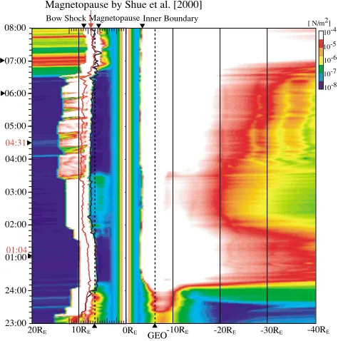
Figure 4 shows the time evolution of the plasma pressure profile,P along the Sun-Earth line. The Earth is located at the origin, and the position of GEO (±6.6RE) is shown by a dotted line. Strong earthward plasma flow appears from 0018 UT in the tail and is accompanied by enhanced mag-netic flux transport. The inner edge of the plasma sheet can be seen by the sharp nightside gradient in plasma pres-sure. It is inside of GEO during this event. Both the bow shock and the magnetopause move in response to the dy-namic pressure and the IMF changes. The bow shock moves

IMF Bz (nT)

31.5

-31.5 31.2

-31.2

IMF By (nT)

51.8

Dp (nP

a)

1.8 -491

V

elocity (km/s)

-658 78.7

Density (/cc)

5.0

Time (UT)

23 00 01 02 03 04 05 06 07 08

23:48 03:16 04:31 06:00

06:40 07:16

B C

A

05:40 07:00

Fig. 2. WIND observations of the solar wind and the IMF from 2300 UT on October 21 to 0800 UT on October 22, 1999. From top to bottom, IMFBzandByin GSM coordinates, the dynamic pressure,Dp, velocity in GSM coordinates, and the number density. A strong southward IMF (Bz= −20 to−30 nT) with a duration of∼6 hours was observed during this period. Moreover, the dynamic pressure of solar wind is in the range from 1.8 to 51.8 nPa.

earthward to about 11.5RE, and the magnetopause shifts to

X =7.2REfrom the Earth when the initial pressure waves hits the magnetosphere at 2315 UT. They again move to-ward the Earth when the IMF turns southto-ward at 2348 UT. The inner edge of the plasma sheet moves toX = −5.5RE following the southward turning.

By 0104 UT when AL reaches−1357 nT, the bow shock approached X = 9.7 RE, while the magnetopause shifts to X =6.5 RE, at this time the inner edge of the plasma sheet reaches up to X = −3.2 RE. Since X = −3.2 RE is very close to the inner boundary of the simulation box,

|X| =2.5 RE, the inner edge might be much closer to the Earth in reality. At the second AL minimum (−1992 nT at 0431 UT), the bow shock moves out to X =14.4 RE, and the magnetopause shifts to X =7.7 RE but the inner edge of the plasma sheet stays close to X = −3.2 RE. Finally, when the second large pressure increase reaches the Earth (between 0600 and 0700 UT), the bow shock and magnetopause move toward the Earth toX=8.3REandX

=5.4RE, respectively. The inner edge of the plasma sheet stays close toX= −3.2RE.

23/21 00/22 01/22 02/22 03/22 04/22 05/22 06/22 07/22 08/22 400

300

200

100

0

-100

-200

Time (UT)

φ(+) − φ(−)

φ(+)

φ(−)

φ

(kV)

23:48 03:16 04:31 06:00 07:00 07:16

B

A C

Fig. 3. Time evolution of the polar cap potential produced by the simula-tion.φ(+),φ(−)andφ(+)−φ(−)are the maximum, the minimum and the cross polar cap potential respectively. The shaded portions indicate characteristic times during this storm event. The cross polar cap poten-tial reaches∼300 kV during the interval from 2300 UT on October 21 to 0800 UT on October 22, 1999.

Bow Shock Magnetopause Inner Boundary

GEO

01:04 04:31

-30RE

08:00

07:00

06:00

05:00

04:00

03:00

02:00

01:00

24:00

23:00

20RE 0RE -10RE -20RE -40RE

10-4

10-8 10-6 [ N/m2]

10-7 Magnetopause by Shue et al. [2000]

10RE

10-5

Fig. 4. Time evolution of the plasma pressure profile along the Sun-Earth line. The Earth is located at the origin, the position of GEO located at ±6.6RE is shown by dotted lines. Positions of the magnetopause by the Shueet al.(2000) are plotted as the thick black (Bz =0) and red (Bz=0) lines.

the IMFBzcomponent is non-zero, the magnetopause shifts earthward 2-3REin distance in comparison with the case of

01:04

04:31

08:00

07:00

06:00

05:00

04:00

03:00

02:00

01:00

24:00

23:00

20RE 10RE_GEO 0RE _GEO-10RE -20RE -30RE -40RE

0 1.5

-1.5 1 0.5

-0.5 -1 [10-2 V/m]

Fig. 5. Time evolution of electric field (Ey) along the Sun-Earth line. The red colors give positive or dawn to dusk electric field (Ey>0) and the blue colors give negative or dusk to dawn electric field (Ey<0).

zero Bz. The difference could come from the effect of the strong southward IMF. There is good agreement between the position of the simulated magnetopause and that of the Shue’s magnetopause model (black line). However, the po-sition of the simulated magnetopause shifts more earthward after 0640 UT. This additional erosion is attributable to the dayside reconnection for the strong IMFBycomponent.

Figure 5 shows the time evolution of the electric field,

Ey=Vx×Bz, on the Sun-Earth line from 2300 UT on Oc-tober 21 to 0800 UT on OcOc-tober 22. The red color indicates positive values of Ey(dawn to dusk) and the blue color in-dicates negative values. A near-Earth neutral line (NENL) appears around X = −10 RE as a gap between two en-hanced regions ofEyin the tail. A high dawn to dusk elec-tric field appears after 0015 UT on the nightside because of the strong southward IMF (Bz = −23 nT at 0015 UT). This is 49 minutes before the time when the first electro-jet minimum is reached at 0104 UT. The duskward electric field is enhanced at 0335 UT and penetrates inside GEO after the arrival of a more southward IMF Bz at 0316 UT. Then 51 minutes later, the second electrojet minimum oc-curs (−1992 nT at 0431 UT). Ey becomes very large at 0640 UT on the nightside, in response to the IMFBz mini-mum (−31 nT) at 0556 UT. Dst reaches its minimum value of−237 nT between 0600 and 0700 UT and the IMF Byis maximum (31 nT) at 0631 UT. The high duskward electric field, Ey, is maintained on the nightside even though IMF

Bz has near zero value. IMF By is duskward with a large value of 21 nT at 0718 UT.

When Ey is 6.5×10−3 V/m (Vx = −466 km/s, Bz =

103 102 1 [eV] 104

Plasma flow

Plasma flow

(a)

30RE

X

Z

Y 30RE

Y Z 30RE

X

30RE

(b)

X = -6.6RE

Magnetopause

-120RE Bo

w Shock

Bo w Shock

Magnetopause

30RE

-30RE

Y 30RE

Z 30RE

10 10-1 -120RE

Fig. 6. Simulation results showing the kinetic energy at 0540 UT (top panel) and at 0640 UT (bottom panel). On the left, the upper (lower) half shows the simulation results inX Z(X Y)plane. The right hand panels are cross sections of the plasma sheet atX= −6.6RE.

(b)

(a)

GEO

Z

Y X Z

X

Energy Flux

Convection Potential

00

06 12

18

70 60 50 40 30

18 19 20 21 22

103 102 10 1 10-1 10-2 10-3

T

L

M

m

c/

gr

e

2

rt

s

c

es

LAT TED flux

(a)

(b)

40 o 50

o 60

o 70

o 80

o

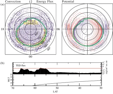
Fig. 8. (a) (left) Convection pattern and energy flux, and (right) polar-cap potential mapped onto the ionosphere obtained by the MHD simulation. The bottom panel (b) is the downward electron energy flux at energies of 0.02−20 keV observed by the TED instrument from the NOAA-15 satellite.

is almost 20% in the outer plasma sheet while the IMFBzis strongly southward for 0330−0540 UT. At 0600−0800 UT,

Ey increases between 90% and 200% in the inner plasma sheet due to compression caused by the strong increase of the solar wind dynamic pressure. Thus a convective electric field, which is almost comparable to (or over) that of the solar wind, can penetrate in to the Earth-side of NENL.

Figure 6 shows the kinetic energy (K = 1₂ρV2) from the simulation (a) at 0540 UT and (b) at 0640 UT. In the left panel, the values in the noon-midnight meridian are plotted on the upper half (X Z) while equatorial values are found on the lower half (X Y). The right hand panels are cross sec-tions of the plasma sheet atX= −6.6RE. We see the loca-tions of the bow shock and the magnetopause in the kinetic energy at the dayside magnetosphere. In the top left the panel, stream-like structure of higher kinetic energy (just below the magnetopause) extends from the cusp toward the mantle. The panel also shows strong tailward plasma flow in the plasma sheet. In the bottom panel (0640 UT), the bow shock and the magnetopause are located closer to the Earth than in the top panel, the whole magnetosphere is com-pressed by a strong increase of solar wind dynamic pres-sure. A large amount of the plasma flows tailward over a wide region of the plasma sheet.

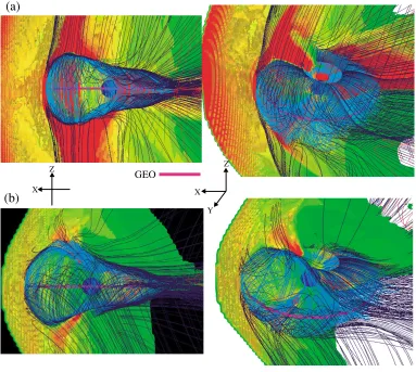
Figure 7 shows a three-dimensional view of the magneto-sphere at two characteristic times. The configuration of the magnetic field lines and the plasma temperature is shown at 0540 UT (a) and 0640 UT (b). The plasma temperature

is shown by 3-D iso-surface only on the dawnside and the color scale is green-yellow-red going from low to high tem-perature. Closed field lines that connect to the Earth in both ends are blue, open field lines that connect to the ionosphere at one end and to the distant IMF at the other are dark blue, and detached field lines (IMF) that do not connect to the Earth at all are red. As shown in Fig. 2, at 0540 UT, the IMF is strongly southward with a smaller dawnwardBy compo-nent (Bz = −31 nT andBy = −1.7 nT). At 0640 UT, the IMFBzis one-third of its former value, and there is a large duskwardBycomponent (Bz = −12 nT andBy =31 nT). The dayside reconnection can be seen atX =7.5RE, and tail reconnection can be found atX = −8.8RE in Fig. 7(a). The dayside reconnection occurs near the GEO region at high-latitudes and tail reconnection is about X = −10RE in Fig. 7(b). The region is verified from theBzprofile along Sun-Earth line. It should be noted that a sharp transition from dipole-like to tail-like magnetospheric configurations occurs near the GEO region in the tail.

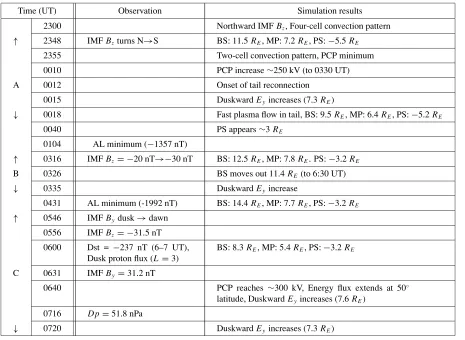
Detec-Table 1. Response of the Earth’s magnetosphere to variations of the solar wind and the IMF. Where BS means the bow shock, MP the magnetopause, PS the inner boundary of plasma sheet, PCP the cross polar cap potential andDpthe dynamic pressure.

Time (UT) Observation Simulation results

2300 Northward IMFBz, Four-cell convection pattern ↑ 2348 IMFBzturns N→S BS: 11.5RE, MP: 7.2RE, PS:−5.5RE

2355 Two-cell convection pattern, PCP minimum

0010 PCP increase∼250 kV (to 0330 UT)

A 0012 Onset of tail reconnection

0015 DuskwardEyincreases (7.3RE)

↓ 0018 Fast plasma flow in tail, BS: 9.5RE, MP: 6.4RE, PS:−5.2RE

0040 PS appears∼3RE

0104 AL minimum (−1357 nT)

↑ 0316 IMFBz= −20 nT→−30 nT BS: 12.5RE, MP: 7.8RE. PS:−3.2RE

B 0326 BS moves out 11.4RE(to 6:30 UT)

↓ 0335 DuskwardEyincrease

0431 AL minimum (-1992 nT) BS: 14.4RE, MP: 7.7RE, PS:−3.2RE

↑ 0546 IMFBydusk→dawn

0556 IMFBz= −31.5 nT

0600 Dst = −237 nT (6–7 UT), Dusk proton flux (L=3)

BS: 8.3RE, MP: 5.4RE, PS:−3.2RE

C 0631 IMFBy=31.2 nT

0640 PCP reaches ∼300 kV, Energy flux extends at 50◦ latitude, DuskwardEyincreases (7.6RE)

0716 Dp=51.8 nPa

↓ 0720 DuskwardEyincreases (7.3RE)

tor (TED) and Medium Energy Proton and Electron Detec-tor (MEPED) are described in Evans and Greer (2000). It should be noted that 1 erg/cm2 sec str could be proxy for visible aurora (Yahninet al., 1997). By 0640 UT, the cross polar cap potential is already increased (Fig. 3), indicating that the convection is enhanced in the ionosphere.

The flow in the throat region (near noon) is poleward on the dayside in the top left panel, and the region of en-hanced energy flux on the dayside is confined in the cusp region. Enhanced nightside energy flux extends as low as 50◦ latitude in simulation. At 19 magnetic local time (MLT), the energy flux appears at 55◦ latitude in simula-tion (Fig. 8(a)), consistent with the low latitude, 52◦of the TED in observation of the NOAA-15 (Fig. 8(b)). On the right of Fig. 8(a), the red contour indicates positive po-tential and blue contour indicates negative popo-tential. The positive potential peak moves tailward in comparison with negative potential due to the large positive By component. The green lines delimit the open-closed field boundary. The open-closed boundary extends at 60◦on the nightside, 72◦ on the dayside, 62◦on dawn, and 66◦on dusk. The 66◦ lat-itude of the open-closed boundary at 17 MLT is consistent with the high-latitude boundary of the TED flux enhance-ment region, which should correspond to the high-latitude boundary of the auroral oval.

5.

Chronology of the Magnetic Storm

We divide these simulation results into three characteris-tic time intervals: when Bz turns from northward to south-ward, when Bz becomes more southward, and when Bz turns from southward to northward. The three characteristic intervals correspond to the shaded portions of A, B, and C in Figs. 2 and 3. The storm event timings are summarized in Table 1.

5.1 Interval A: IMFBzturns from northward to

south-ward (2330-0020 UT)

When the IMF turns from northward to southward at 2348 UT, the initial four-cell convection pattern in the po-lar ionosphere gradually changes to a two-cell convection pattern. The cross polar cap potential increases up to 300 kV and the convective flow increases on the dayside. Fast plasma flow is generated in the plasma sheet just 6 minutes after the onset of tail reconnection at 0018 UT. In this time, the Alfv´en Mach number,MA = Vsw/VA =8.47, and the bow shock moves toX =9.5RE, while the magnetopause shifts toX =6.4RE and the inner edge of the plasma sheet moves to the Earth toX = −5.2 RE.

5.2 Interval B: IMF Bz becomes more southward

(0300-0340 UT)

de-6

290 292 294 296 298 300

Kp

Fig. 9. (a)Lvalue with time diagram for the proton flux, represented by the color code.The trapped proton flux is observed in the duskside. The red line is location of the plasmapause, while the black line is the reference line to represent the variation of the convection limit. (b) Kp and (c) Dst indices are represented on the lower two panels.

creases in the dayside region because the dynamic pressure of the solar wind decreases. Due to the effect of the de-creases in pressure and the low Mach number (MA=2.42), the bow shock moves out to X =14.4 RE, while the mag-netopause shifts to X = 7.7 RE and the inner edge of the plasma sheet close toX = −3.2RE.

5.3 Interval C: IMFBzturns from southward to

north-ward (0540−0720 UT)

During this interval, IMF Bz is still strongly southward (∼−30 nT) until 0630 UT, and then IMFBzbecomes more northward. The IMFByis a large positive value and the dy-namic pressure increases, the energy flux in the ionosphere increases on the dayside and the cross polar cap potential remains constant at a high value of 300 kV. The duskward electric field increases on the nightside from 0640 UT. The bow shock approaches to X = 8.3 RE, while the magne-topause shifts to X = 5.4 RE and the inner edge of the plasma sheet stays atX = −3.2 RE.

6.

Discussion

In this paper, we have studied the response of the Earth’s magnetosphere to variations in the solar wind and the IMF. The strong magnetic storm event of October 21 and 22 could be well represented even in the near-Earth magne-totail region by this simulation.

The cross polar cap potential increases and reaches a maximum at 0010 UT, 16 minutes after the IMF turns from northward to southward. The response of the magneto-sphere takes a short time from variations of the solar wind. The time is considered to be 4–6 min to allow for the prop-agation of the solar wind from the WIND position to the Earth. Note that the substorm occurs in the tail accompa-nied with a strong earthward flow, caused by the enhanced convection (duskward Ey increases) due to the tail recon-nection.

Figure 9 shows theL value-time spectrogram for 30–80 keV proton flux from the MEPED instrument the NOAA-15. This energy has been considered as the main part of ring current. The trapped proton flux observed in the dusk

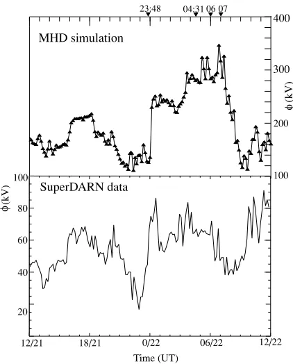
(kV)

(kV)

Time (UT)

MHD simulation

SuperDARN data

12/21 18/21 0/22 06/22 12/22

100 100

Fig. 10. Comparison between the cross polar cap potential pattern from the MHD simulation and that inferred from the SuperDARN observations.

side is in panel (a). The Kp (b) and Dst (c) indices are rep-resented on the lower two panels. The red line is the loca-tion of the plasmapause evaluated from the empirical rela-tion as a funcrela-tion of the Kp index by O’Brien and Moldwin (2003). The black is also derived from the same relation-ship, but the refilling time of plasmasphere is not consid-ered. Thus, it is supposed that the black line can be a proxy for activity of magnetospheric convection. The proton flux enhancement is observed when the magnetic storm at lower

L value,L < 3, in the NOAA-15 data. This implies that the inner boundary of the plasma sheet moves toward the Earth concurrently with the convection enhancement, and such movement of the plasma sheet can be clearly seen in our simulation (cf. Fig. 4).

We also have compared our simulation results of the polar cap potential with the SuperDARN observations in Fig. 10. The simulated cross polar cap potential is∼3−4 times larger than that inferred from the SuperDARN ob-servations. However the characteristic timings of the increase and decrease in the potential are similar from 1200−2100 UT on October 21. The second method in Sec-tion 2.3 that we use to obtain the polar cap potential, in principle, does not depend on the ionospheric conductivity because the feedback effect is neglected. It is noted that the cross polar cap potential obtained gives the maximum generated by the inner magnetospheric convection. There-fore, the polar cap potential in reality can be less than that given in the present simulation. The polar cap potential de-pends on the ionospheric conductivity due to the feedback effect. The difference of magnitude of the polar cap poten-tial needs further study comparing the two methods to give the magnetosphere-ionosphere relationship.

the SuperDARN observation increased just after the IMFBz turned from northward to southward at 2348 UT. The simu-lated cross polar cap potential reached 300 kV, whereas the SuperDARN observations give only about 68 kV. The polar cap potential in simulation is almost constant with 250 kV during the strong southward IMFBz(−20 nT) for 3 hours at 0100-0300 UT. Then it increases from 250 to 300 kV when the IMF Bzis more southward from−20 to−30 nT at 0300-0600 UT. The time variation is similar to that of the PC index (e.g., Troshichevet al., 1996). On the other hand, the potential shown from SuperDARN observations quickly decreases from 0015 UT on October 22 and then it did not increase so strongly at 0300−0600 UT on Octo-ber 22. This result comes from the increased ionospheric conductivity due to the enhanced of the magnetospheric convection and the field-aligned currents. The dense par-ticle precipitation in the nightside (e.g., DMSP data) leads to the increase in ionospheric conductivity, and the poten-tial is sensitive to the conductance (Richmondet al., 1988; Richmond, 1992). Thus the polar cap potential of the Su-perDARN quickly decreases. Moreover, the SuSu-perDARN potential is not so much increased for the strong southward IMFBz(∼−30 nT), partly because of insufficient data cov-erage during the strong magnetic storm period.

The cross polar cap potential saturates for a strong Bz component. Siscoeet al.(2002) proposed that the saturation of the polar cap potential originated from the ionospheric conductivity and region 1 current limitation by ram pres-sure. Merkineet al.(2003) showed, by using global MHD modeling, that the potential saturated as the solar wind electric field increased, and that the saturation level was strongly affected by the ionospheric conductance. However, the saturation mechanism (Interval B) in this event study is independent of the ionospheric conductivity, suggesting an-other possibility of the saturation mechanism. The mecha-nism may be connected to a relative reduction of the day-side magnetic reconnection rate. We find in our simulation that the reconnected open field lines at the dayside mag-netopause is almost parallel to the IMF. The reconnected field line are not fully carried away from the reconnection region due to very strong southward IMF and normal solar wind speed. Therefore, the reconnection rate does not re-markably increase even though IMF Bz decreases down to

−30 nT.

The cross polar cap potential in the simulation is main-tained at a large value even when the IMF Bz becomes less negative or even positive. This is caused by the large IMF By at this time (Fig. 2), and the IMF lines can di-rectly approach reconnection regions at the dayside mag-netopause close to the Earth. The dayside reconnection oc-curs at high latitudes in the northern dusk sector close to the GEO with naked geomagnetic field lines because of the large duskward IMFBycomponent at 0640 UT. Therefore, the convection enhancement in the ionosphere appears and leads to a large value of the cross polar cap potential.

7.

Conclusions

We have used a three-dimensional global MHD model to simulate the interaction of the solar wind with the Earth’s magnetosphere to study a strong magnetic storm on

Octo-ber 21–22, 1999, when the IMF was strongly southward (Bz = −20 to−30 nT) for∼6 hours. The dynamic pressure of the solar wind was in the range 1.8−51.8 nPa during this period. The simulation reproduced the time evolution of the cross polar cap potential, the kinetic energy, the plasma pressure,Ey, and the locations of the bow shock, the mag-netopause, and the inner edge of plasma sheet in this event. The following conclusions can be obtained from the present simulation:

1) As the IMF is strongly southward (−20 nT to−30 nT) for 6 hours, the geomagnetic field lines in the day-side magnetopause are eroded to the GEO region by reconnection. Moreover, the associated magnetic flux is transferred from the dayside magnetosphere to the tail. Reconnection still occurs near the GEO region on the dayside magnetopause (Fig. 7(b)), even though the IMFBzcomponent becomes small or even turns to northward, because of the influence of the following a strong IMF By (30 nT). During the large By inter-val, the IMF lines can reconnect the naked geomag-netic field with a large magnitude in the high-latitude flanks. Thus the cross polar cap potential is maintained at a large value and the convection in the ionosphere is enhanced. The cross polar cap potential is governed by IMFByas well asBz components. It saturates for the strong southward IMF (φ∼250 kV forBz∼ −20 nT andφ ∼300 kV for Bz ∼ −30 nT). Potential satura-tion may be connected to relative reducsatura-tion of the day-side magnetic reconnection rate. We find in our simu-lation that the reconnected open field lines at the day-side magnetopause are almost parallel to the IMF. The reconnected field lines are not fully carried away from the reconnection region for very strong southward IMF and normal solar wind speed. Therefore, the recon-nection rate does not increase remarkably, even though IMFBzdecreases down to−30 nT.

2) The dynamic pressure of the solar wind shows a spiky peak for a short interval (about 10 minutes), however it has a rather small effect on the cross polar cap po-tential increases as both the absolute values of IMFBy and IMFBzare gradually decreasing at that time. En-hanced energy flux appears at low latitude (50◦) on the nightside in simulation. The energy flux in the region 19 MLT, appears down to a 55◦ latitude in simulation and is consistent with the low latitudes, 52◦of the ener-getic electrons from the NOAA-15 satellite. The open-closed boundary extends to lower latitudes at 60◦ on the nightside, 72◦ on the dayside, 62◦ on dawn, and 66◦on dusk. The 66◦latitude on dusk from the simu-lation is consistent with the high-latitude boundary of TED flux enhancement region.

3) The initial plasma pressure change leads to a strong earthward flow at 0040 UT in the simulation. This is the start of a substorm and is consistent with the de-crease in the AL index, corresponding to the develop-ment of auroral electrojet current (Fig. 1).

close to−3.2 RE at the time when the dynamic pres-sure of the solar wind reaches its maximum value at

∼0700 UT. At the same time, Ey increases by 90– 200% in the inner plasma sheet due to compression by the strong increase of the solar wind dynamic pressure. The convective electric field, which is almost compara-ble to (or larger than) that of the solar wind, penetrates into the Earth-side of NENL.

We have obtained the magnetospheric configuration and dynamics for a event study of a strong magnetic storm. The large energy flux enters the ionosphere at very low latitudes and the inner edge of the plasma sheet becomes very close to the Earth for a strong magnetic storm. These results are consistent with the observation data. The present MHD simulation study gave reasonable results in near-Earth mag-netotail dynamics even for extreme conditions and thereby its usefulness could be demonstrated as a physical model for space weather studies.

Acknowledgments. We would like to thank Raymond J. Walker, Hiroyuki Shinagawa, Yoshizumi Miyoshi, Yukinaga Miyashita and Kazuo Shiokawa for helpful discussions A. T. Y. Lui for pro-viding the polar cap potential data and Nozomu Nishitani for use-ful discussion on the potential maps from the SuperDARN radars in the northern hemisphere. The WIND data of solar wind and magnetic field in ISTP Key Parameters were provided courtesy of Drs. K. W. Ogilvie and R. P. Lepping respectively. The ge-omagnetic indices AL, AU and Dst were provided by the WDC for Geomagnetism in Kyoto. The data from the NOAA satellites were provided by NOAA through the WDC-C2 for Aurora, Na-tional Institute of Polar Research, Japan. Computing support was provided by the Information Technology Center of Nagoya Uni-versity. Support was provided by Grants-in-Aid from the Japan Society for Promotion of Science (JSPS).

References

Ashour-Abdalla, M., M. El-Alaoui, V. Peroomian, R. J. Walker, L. M. Zelenyi, L. A. Frank, and W. R. Paterson, Localized reconnection and substorm onset on Dec. 22, 1996,Geophys. Res. Lett.,26, 3545–3548, 1999.

Ashour-Abdalla, M., M. El-Alaoui, F. V. Coroniti, R. J. Walker, and V. Peroomian, A new convection state at substorm onset: Results from an MHD study,Geophys. Res. Lett.,29, 1965, 2002a.

Ashour-Abdalla, M., M. El-Alaoui, V. Peroomian, R. J. Walker, L. M. Ze-lenyi, L. A. Frank, and W. R. Paterson, The origin of the near-Earth plasma population during a substorm on November 24, 1996,J. Geo-phys. Res.,105, 2589–2605, 2002b.

Brecht, S. H., J. G. Lyon., J. A. Fedder, and K. Hain, A simulation study of east-west IMF effects on the magnetosphere,Geophys. Res. Lett.,8, 397–400, 1981.

Evans, D. S. and M. S. Greer, Polar orbiting environmental satellite space environment monitor: 2. Instrument description and archive data docu-mentation,NOAA Tech. Memo. OAR SEC-93,Natl. Oceanic and Atmos. Admin., Boulder, Colo., 2000.

Fedder, J. A. and J. G. Lyon, The solar wind-magnetosphere-ionosphere current-voltage relationship,Geophys. Res. Lett.,14, 880–883, 1987. Fedder, J. A., S. P. Slinker, J. G. Lyon., and R. D. Elphinstorne, Global

numerical simulation of the growth phase and the expansion onset for a substorm observed by Viking,J. Geophys. Res.,100, 19083–19093, 1995.

Le, G., J. Raeder, C. T. Russell, G. Lu, S. M. Petrinec, and F. S. Mozer, Polar cusp and vicinity under strongly northward interplanetary

mag-netic field on April 11, 1997: Observations and MHD simulations,J. Geophys. Res.,106, 21083–21093, 2001.

Lui, A. T. Y., R. W. McEntire, and K. B. Baker, A new insight on the cause of magnetic storms,Geophys. Res. Lett.,28, 3413–3416, 2001. Lyon, J. G., S. H. Brecht, J. D. Huba, J. A. Fedder, and P. J. Palmadesso,

Computer simulation of a geomagnetic substorm,Phys. Rev. Lett.,46, 1038–1041, 1981.

Lyons, L. R., The Geospace Modeling Program Grand Challenge,J. Geo-phys. Res.,103, 14781–14785, 1998.

Lyons, L. R., J. M. Ruohoniemi, and G. Lu, Substorm-associated changes in large-scale convection during the November 24, 1996, Geospace Environment Modeling event,J. Geophys. Res.,106, 397–405, 2001. Merkine, V. G., K. Papadopoulos, G. Milikh, A. S. Sharma, X. Shao, J.

Lyon, and G. Goodrich, Effects of the solar wind electric field and ionospheric conductance on the cross polar cap potential: Results of global MHD modeling,Geophys. Res. Lett.,23, 2180, 2003.

O’Brien, T. P. and M. B. Moldwin, Empirical plasmapause models from magnetic indices,Geophys. Res. Lett.,30, 1152, 2003.

Ogino, T., R. J. Walker, M. Ashour-Abdalla, and J. M. Dawson, An MHD simulation of By-dependent magnetospheric convection and field-aligned currents during northward IMF, J. Geophys. Res., 90, 10835–10842, 1985.

Ogino, T., R. J. Walker, and M. Ashour-Abdalla, A global magnetohydro-dynamic simulation of the magnetosheath and magnetosphere when the interplanetary magnetic field is northwards,IEEE Trans. Plasma Sci., 20(6), 817, 1992.

Raeder, J., J. Berchem, and M. Ashour-Abdalla, The Geospace Environ-ment Modeling Grand Challenge: Results from a global geospace circu-lation model,J. Geophys. Res.,103, 14787–14797, 1998.

Raeder, J., R. L. McPherron, L. A. Frank, S. Kokubun, G. Lu, T. Mukai, W. R. Paterson, J. B. Sigwarth, H. J. Singer, and J. A. Slavin, Global simulation of the Geospace Environment Modeling substorm challenge event,J. Geophys. Res.,106, 381–395, 2001.

Richmond, A. D., Y. Kamide, B.-H. Ahn, S.-I. Akasofu, D. Alcayde, M. Blanc, O. de la Beaujardiere, D. S. Evans, J. C. Foster, E. Friis-Christensen, T. J. Fuller-Rowell, J. M. Holt, D. Knipp, H. W. Kroehl, R. P. Lepping, R. J. Pellinen, C. Senior, and A. N. Zaitzev, Mapping elec-trodynamic features of the high-latitude ionosphere from localized ob-servations: Combined incoherent-scatter radar and magnetometer mea-surements for January 18–19, 1984,J. Geophys. Res.,93, 5760–5776, 1988.

Richmond, A. D., Assimilative mapping of ionospheric electrodynamics,

Adv. Space Res.,12, 59–68, 1992.

Shue, J.-H., P. Song, C. T. Russell, J. K. Chao, and Y.-H. Yang, Toward predicting the position of the magnetopause within geosynchronous orbit,J. Geophys. Res.,105, 2641–2656, 2000.

Siscoe, G. L., N. M. Crooker, and K. D. Siebert, Transpolar potential saturation: Role of region 1 current system and solar wind ram pressure,

J. Geophys. Res.,107, 1321–1328, 2002.

Slinker, S. P., J. A. Fedder, J. M. Ruohoniemi, and J. G. Lyon, Global MHD simulation of the magnetosphere for November 24, 1996,J. Geophys. Res.,106, 361–380, 2001.

Troshichev, O., H. Hayakawa, A. Matsuoka, T. Mukai, and K. Tsuruda, Cross polar cap diameter and voltage as a function of PC index and interplanetary quantities,J. Geophys. Res.,101, 13429–13435, 1996. Walker, R. J., T. Ogino, J. Raeder, and M. Ashour-Abdalla, A global

mag-netohydrodynamic simulation of the magnetosphere when the interplan-etary magnetic field is southward: the onset of magnetotail reconnec-tion,J. Geophys. Res.,98, 17235–17246, 1993.

Watanabe, K. and T. Sato, Global simulation of the solar wind-magnetosphere interaction: The importance of its numerical validity,J. Geophys. Res.,95, 75–88, 1990.

Yahnin, A. G., V. A. Sergeev, B. B. Gvozdenvsky, and S. Vennerstrom, Magnetospheric source region of discrete auroras inferred from their relationship with isotropy boundaries of energetic particles,Ann. Geo-phys.,15, 943–958, 1997.