R E S E A R C H
Open Access
A splitting algorithm for a novel
regularization of Perona-Malik and application
to image restoration
Fahd Karami
*, Lamia Ziad and Khadija Sadik
Abstract
In this paper, we focus on a numerical method of a problem called the Perona-Malik inequality which we use for image denoising. This model is obtained as the limit of the Perona-Malik model and thep-Laplacian operator with p→ ∞. In Atlas et al., (Nonlinear Anal. Real World Appl 18:57–68, 2014), the authors have proved the existence and uniqueness of the solution of the proposed model. However, in their work, they used the explicit numerical scheme for approximated problem which is strongly dependent to the parameterp. To overcome this, we use in this work an efficient algorithm which is a combination of the classical additive operator splitting and a nonlinear relaxation algorithm. At last, we have presented the experimental results in image filtering show, which demonstrate the efficiency and effectiveness of our algorithm and finally, we have compared it with the previous scheme presented in Atlas et al., (Nonlinear Anal. Real World Appl 18:57–68, 2014).
Keywords: Image restoration, Perona-Malik inequality,p-Laplacian, Splitting algorithm
1 Introduction
Image denoising is one of the fundamental challenges in the field of image processing and computer vision. The aim is to remove noise while preserving edges, boundaries, and textures. To handle this problem, partial differential equations [1–7], variational models [8–11], energy minimization, bilateral filtering [12, 13], and wavelet thresholding [14, 15] have been proposed depend-ing on the domain of applications. Generally, the partial differential equations use a nonlinear anisotropic diffu-sion to restore a degraded image which they seek to improve its quality by removing noise while preserving details and even enhancing edges.
In 1990, Perona-Malik [2] proposed a nonlinear dif-fusion equation that succeeded in image denoising. Although, this model is an ill-posed problem in ana-lytical point of view, besides, the numerical simulations produce the staircase effect. This paradoxical result has been named as the Perona-Malik Paradox [16]. Motivated by the ill-posedness of the Perona-Malik model, many
*Correspondence: [email protected]
Université Cadi Ayyad, Ecole Supérieure de Technologie d’Essaouira, B.P. 383 Essaouira El Jadida, Essaouira, Morocco
works (see for instance [17–19]) suggest to introducing the regularization in space and/or time. Using the spatial convolution inside the anisotropic diffusion and replacing the diffusivity by a slight variation, new modified mod-els have been proposed, but they produce an undesirable blurring effect. Otherwise, some new class of backward-forward regularizations has been introduced. In [20], the authors combine the Perona-Malik with a Laplacian oper-ator and develop a new effective model, and they make a generalization of their results by replacing the Laplacian with a nonlinearp-Laplacian operator forp ∈ (1, 2] (cf. [21]). Recently, in [22], the authors proposed a new regu-larization based on the previous interpolation of Perona-Malik andp-Laplacian with large value ofp. Their model is well posed, it reduces the staircase effect and avoids creating new features in the image, they have also done a study of the limiting problem. For a numerical purpose, the authors used an explicit finite difference scheme which is unstable and the condition of stability depends on the parameterp.
In this paper, we develop a numerical semi-implicit method approaching the Perona-Malik inequality by using
minimization problem [25].
The rest of this paper is organized as follows. In the next Section 2, we provide reviews of some previous works that are Perona-Malik model,p-Laplacian equation and their interpolation. In Section 3, we present a new numerical scheme using an operator splitting algorithm that splits the Perona-Malik inequality in two sub-models treated by additive operator schemes and dual formulation, respec-tively. Finally, some numerical simulations are given to demonstrate the effectiveness of the proposed algorithm.
2 Reviews of some previous works
In this section, we recall some previous models. LetT >0 be a fixed time,f the intensity of the noisy image,u the desired clean image that was corrupted with the noisen
such thatf = u + n, and letbe a bounded picture domain with smooth boundary.
2.1 Perona-Malik model
The Perona-Malik model is a powerful model and widely used in image denoising. Hence, the idea behind this model is to improve the results obtained by the PDE heat and to change the equation by introducing the edge detec-tion process (the diffusivity coefficient). Perona-Malik problem is obtained by solving the following anisotropic diffusion equation with a Neumann boundary condition:
⎧ ⎨ ⎩
ut− div
g(|∇u|)∇u=0 in Q:=(0,T)×,
∇u.n=0 in:=(0,T)×,
u(x, 0)=f in.
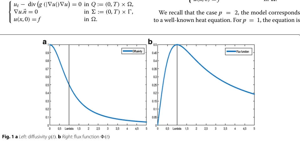
whereλ >1 is a threshold parameter that determines the size of the gradients which will be preserved and g is a decreasing function worthλwhere|∇u|is close to 0 and tend to 0 for large|∇u|. Note that ifg(.) ≡1, we recover the heat equation. For the diffusivity functiong, it follows the flux function(t) = tg(t)which satisfies(t) ≥ 0 for|t| ≤λand(t)≥0 for|t| ≤λ.
We observe from the Fig. 1b that the Perona–Malik model is a forward parabolic type for|t| ≥ λand a back-ward parabolic type for|t| ≤λ. This model is an ill-posed problem from the mathematical point of view and pro-duces an unwanted phenomena well known by staircase effect.
2.2 Thep-Laplacian equation
To obtain the p-Laplacian equation, we merely replace the diffusion functiongof the Perona–Malik equation by
g(t)=tp−2. Thep-Laplacian equation has been proposed and studied by many authors (see for instance [26]). It plays an important role in the modeling of many phenom-ena in different areas such as image processing [27], sand-pile [28, 29], and fluid mechanic [30]. The evolutionary
p-Laplacian equation can be written as: ⎧
⎨ ⎩
ut−div
|∇u|p−2∇u=0 inQ,
∇u.n=0 in,
u(x, 0)=f in.
We recall that the casep = 2, the model corresponds to a well-known heat equation. Forp = 1, the equation is
Fig. 2Images corrupted by Gaussian noise with zero mean and varianceσ2 = 0.025
called total variation and for a largep, the model is known as the infinite Laplacian.
2.3 Perona-Malik andp-Laplacian model
The staircasing phenomena is a manifestation of the forward-backward nature of the Perona-malik equation which appears in its discretization. In order to escape the backward regime, a novel kind of regularization [20–22] of the classical Perona-Malik model is proposed for image processing. This regularization still allows gradi-ent growth while controls its maximal size which is done by combining two classical models, Perona-Malik and
p-Laplacian.
Indeed, the following regularization reduces the size of the backward region and the solutions can flee the backward region simply by developing small and large gradients:
⎧ ⎨ ⎩
ut− div
g(|∇u|)∇u− λ1pdiv
|∇u|p−2∇u=0 inQ,
∇u.n=0 in,
u(x, 0)=f in.
(1)
This problem is well posed for a largep, and the exis-tence and uniqueness of the asymptotic behavior asp→
∞are established in [22]. Lettingp→ ∞, the problem (1) converges to the following model:
⎧ ⎨ ⎩
ut−div
g(|∇u|)∇u+∂IK(u)0 inQ
∇u.n=0 in,
u(x, 0)=f in,
(2)
where
K = φ∈W1,r() : | ∇φ| ≤λa.e. in,
andIK(.)denotes the indicator functional of the setK, for allu∈W1,r()IK is defined by:
IK(u)=
0 if u∈K, +∞ if u∈/K.
Thanks to Remark 3.2 of [22], for p > λ2 + 1, the problem (1) has a unique weak solutionupand
forp→ ∞, up→uweakly inLr(0,T,W1,r()) for allr>1.
Moreover,u ∈ W∩Ktis the unique solution of (2) in the following sense:
T
0
∂
u ∂t,u−φ
dt+
T
0
g(|∇u|)∇u∇(u−φ)≤0,
for anyφ ∈ Kt = {ξ ∈ Lr(0,T;W1,r()) : ξ(t) ∈ K}, having
W=
φ ∈Lr0,T;W1,r(): ∂φ ∂t
∈Lr0,T;(W1,r()) ,r>1.
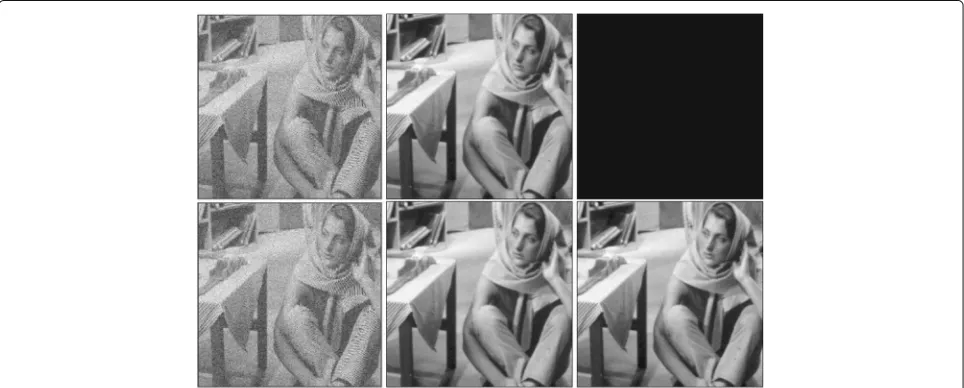
Fig. 4Left column, original images;middle column,noisy images corrupted by poissonian noise;right columnrestored images withλ = 60
For further details and another sophisticated notion of solutions, we refer to [22]. We remark that the limiting problem can be rewritten as:
ut−divg(|∇u|)∇u−f ≤0, |∇u| ≤λ,
ut−div
g(|∇u|)∇u−f(|∇u| −λ)=0,
which is equivalent to solving the Perona-Malik problem in the region where the norm of the gradient is less thanλ.
3 An operator splitting algorithm
The operator splitting methods are very useful to derive fast algorithms. It is worthwhile to be used when the prob-lem we want to solve has an additive structure, the main idea is to split the problem into sub-problems that are eas-ier to solve by treating its summands separately in each iteration of the algorithm. To achieve this goal, we use of the operator splitting algorithm that splits the proposed model into two equations. The first one corresponds to solve the following Perona-Malik model:
⎧ ⎨ ⎩
ut−div
g(|∇u|)∇u=0 inQ,
∇u.n=0 in,
u(x, 0)=f in.
(3)
The second is a diffusion equation associated to the infinity Laplacian that is given by:
⎧ ⎨ ⎩
ut+∂IK(u)0 inQ,
∇u.n=0 in,
u(x, 0)=f in.
(4)
Let N > 0 be given,τ = T/N be the time step,
tn = nτ, n = 0,. . .,N, and let us considerun an approximation ofu(tn)for alln = 0,. . .,N.
The basic idea is to discretize the Eq. (2) by using an implicit scheme for linear terms and an explicit scheme for the remaining terms. The goal is to reduce the exe-cution time required to solve the equations by splitting up the terms in such a way that the stable time step for the explicit discretization is significantly smaller than the largest stable time step for the semi-implicit one.
After discretizing (2) with a semi-implicit first order scheme, we should findun+1satisfying:
⎧ ⎨ ⎩
un+1−un
τ −div
g(|∇un|)∇un+1+∂I
K(un+1)0, ∇un+1.n=0,
un=f.
(5)
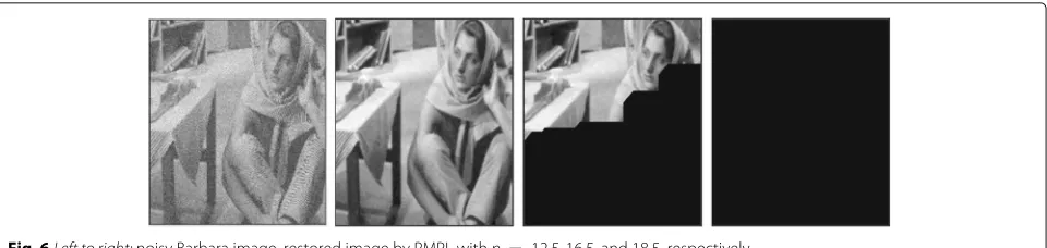
Fig. 6Left to right:noisy Barbara image, restored image by PMPL withp = 12.5, 16.5, and 18.5, respectively
The corresponding discretization of the time splitting scheme (3)–(4) consists on finding at each time step,
vn+12 satisfying:
followed by findingwn+1satisfying: ⎧
The Perona-Malik operator has been solved by differ-ent numerical methods and techniques and methods. To improve computational efficiency, we discretize (3) by (6) and we use the additive operator splitting scheme in the numerical implementation. On the other hand, the sub-differential Eq. (4), discretized by (7), is formulated as a minimization that will be solved by the dual formula-tion [25]. In the sequel, the two numerical methods are presented.
3.1 Perona-Malik operator
The simplest discretization of them-dimensional Eq. (6) with reflecting boundary conditions is given by:
un+ denote, respectively, the approximation of u(xi,tn) and
g(|∇u(xi,tn)|),mis the dimension size andNl(i)consists
of the two neighbors of pixelialong theldirection for all
l = 1,. . .,m. In vector-matrix, notation (8) becomes:
The modification applied to (9) has been introduced firstly by [24] named as additive operator splitting (AOS) scheme which leads us to:
un+12 = 1
3.2 The sub-differential flow
The discretization of the problem (7) can be written as:
wn+1+∂IK(wn+1)wn+ 1
2 forn = 0,. . .,N. (11)
where∂f denotes the sub-differential of a given functionf. Thanks to [25], we focus our attention on the projection
wn+1 = PK
Table 1PSNR and SNR values for the noisy and recovered images corresponding to the experiments shown in Figs. 2 and 3
Images a b c d
PSNR SNR PSNR SNR PSNR SNR PSNR SNR
Noisy 20.1753 8.6159 20.2006 7.8502 20.1582 9.8390 20.1338 2.0217
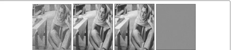
Fig. 7Left to right:noisy image, restored Barbara image by our method, image obtained by PMPL model withp = 20, the difference image
The dual formulation has been used to deal with this minimization problem. The dual problem associated with (12) is given by the following functional:
G(z)=
(div(z))
2 +
w
n+1
2div(z) + λ
|z|. (13)
In order to find the numerical solution of the functional (13), we denote byzha minimizer of this functional and
Gh(zh)the approximation ofG(z)(see [25] for instance):
Gh(zh) =
(div(zh))
2+
w
n+12 h div(zh)
+λ
τ∈Th
|τ||zh(Pτ)|, (14)
whereτrepresents simplex of the partitioning ofTh,|τ|is the area of simplexτ, andPτ is one of the vertices ofτ. In image processing,|τ|could be seen as discretization step
h2 = 1.
In view of the fact thatGh is nondifferentiable, we use a relaxation algorithm (see for instance [31] and the refer-ences therein) to minimize the functional (14) that can be summarized as follows:
1. Initiate the algorithm with vectorq0, setk = 0,
choose a canonical directionej∈Rn. 2. Solving the one-dimensional sub-problems
min
t∈Rjk(t)wherejkis defined as: jk: R→R
t→Gh
qk+tej
. (15)
3. Takingqk+1 = qk+ωtjk, whereω >0is an over-relaxation parameter.
4. We can use Newton algorithm to findtjk, whenjkis differentiable. Else, it can be computed directly. 5. The condition to stop this algorithm is
qk−qk+1l2(Rn)≤ε, for a given convergence toleranceε.
At last, in the next section, results of numerical simula-tions are given.
4 Numerical results and simulations
This section is devoted to extensive numerical experimen-tations. The program will stop when it achieves our goal. Most algorithm parameters are chosen heuristically for the algorithms to perform their best. We set, the spatial sizeh = 1 and the parameter ω = 1, 2 of the relax-ation algorithm. First, we illustrate the efficiency of our proposed numerical algorithm (cf. Figs. 2, 3, 4, and 5) for filtering the images corrupted with noise. As a second experiment, we will keep the same values of the previ-ous parameters and we test the explicit scheme of the Perona-Malik and p-Laplacian (PMPL) proposed in [22] for different values ofpFig. 6. We remark that the PMPL scheme depends on the parameter pand for a large p, the restored image has been damaged. In order to avoid numerical instability, we must take a very small time step. So that, the needed simulation takes more time due to the nature of data. For that, in the third test , we evaluate the performance of our algorithm compared to PMPL scheme
Table 2CPU time of our algorithm and PMPL method for the Barbara and rice images
Images Barbara Rice
Our method 132.86 ×10³ ms 27.30× 10³ ms
Explicit schemes 541.82 ×10³ ms 121.02 ×10³ ms
by using CPU time. The last experiment aims to show the dependence also of the PMPL scheme to the threshold parameterλ.
For the improvements tests, we present the restora-tions and the results of our algorithm by choosing the parameterλ = 20.
The restored images are clearly better than the noisy ones; to obtain an objective evaluation of the proposed method, the peak signal-to-noise ratio (PSNR) is used to measure the quality of the restoration results which is defined as:
PSNR=10 log10
2552MN
||u0−u||22
dB,
where u0, u, and M × N are the original image, the
restored image and the size of the image, respectively. To qualify the restoration capacity of the method under con-sideration, the signal-to-noise ratio (SNR) is applied and denoted by:
SNR=log10 σ
u σn
dB,
whereσuandσnare the signal and noise standard devia-tions, respectively. The value of these statistical measures
indicates the strength of signal in restored images. There-fore, the value increases as the restored version of the image approaches the original one. In order to better eval-uate the restoration process, PSNR and SNR values are shown in the Table 1.
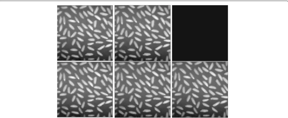
Now, we are testing our method on Barbara and Rice images corrupted by Gaussian noise with zero mean and varianceσ2=0.03 and using the same parameters (Fig. 5). The previous tests show the efficiency of our method. To argue the usage of the proposed algorithm, we will test, in the second experiment, the PMPL model using the explicit scheme proposed in [22] by using the same parameters of the previous test. We take different values ofpto study its impact on the image restoration.
Figure 6 shows that the PMPL method has restored the image, but whenpbecomes large, the images are damaged due to the problem of stability which depends on the value of the parametersp andλas well as the initial data. In order to repair the image and avoid numerical instability, we increase the value of the parameterλand decrease the time step sizedt until finding a suitable value for which the image will not get damaged. In this case, the PMPL scheme becomes stable for dt = 10−3andλ = 60. In Figs. 7 and 8, we will fixλ = 60 and we present the comparison between our algorithm withdt = 0.1 and the PMPL method withdt = 10−3(Fig. 6).
The Figs. 7 and 8 show that the two methods give similar results. But in this experiment, our algorithm has restored the images in fewer time compared to the PMPL method (Table 2).
In the last test, we keep the same parameters employed in the previous experiment and change the value of the thresholdλ(Figs. 9 and 10).
Fig. 10Top row, restored Rice image by PMPL method;bottom row, restored images by our algorithm; first column, noisy images; two right columns, recovered withλ=29.05 andλ=29, respectively
In this experiment, the proposed algorithm proves to be performing better than the explicit scheme where the restored images are damaged when we took a λ small and/orplarge (Fig. 9). The results of this section confirm the usefulness of our method that overcomes the condi-tion of stability; whereas, we remark that for the explicit scheme, the stability criterion is given by dt ≤ f(p,λ) wheref is a decreasing function with respect topand a nondecreasing with respect toλsuch that
f(p,λ)−→0 asp→ ∞andf(p,λ)−→0 asλ→0.
5 Conclusions
Perona and Malik proposed one of the pioneering model which represents an efficient and effective tool for image denoising. However, the numerical simulations produce a phenomenon known as the staircase effect, which causes images to look blocky. To overcome this, in [22], we have proposed a regularized model which is an interpolation of two classical models, Perona-Malik andp-Laplacian with
p → ∞. We have also demonstrate the efficiency and effectiveness of this model compared with the method most frequently used (see [22] for more detail). However, a major drawback for the numerical scheme is that the sta-bility condition is strongly dependent to the parameters
p,λ, anddt. For that, in this work, we develop a novel algo-rithm based on fractional step methods. Combining the classical additive operator splitting and a nonlinear relax-ation algorithm, the numerical experiments demonstrate that the proposed algorithm is accurate and effective for images restoration. Comparing with the classical explicit schemes presented in [22] which strongly depends on the regularization methods and the model parameters,
our algorithm controls the problem of stability and is significantly faster.
Acknowledgements
The authors gratefully acknowledge the helpful comments and suggestions of the reviewers, which have improved the presentation.
Author’s contributions
All authors contributed equally to this work. All authors read and approved the final manuscript.
Competing interests
The authors declare that they have no competing interests.
Publisher’s Note
Springer Nature remains neutral with regard to jurisdictional claims in published maps and institutional affiliations.
Received: 12 January 2017 Accepted: 29 May 2017
References
1. M Arian, N Manjari, B Richard, Anisotropic nonlocal means denoising. Appl. Comput. Harmon. Anal.35, 452–482 (2013)
2. P Perona, J Malik, Scale-space and edge detection using anisotropic diffusion. IEEE Trans. Pattern Anal. Mach. Intell.12(7), 629–639 (1990) 3. Y Wang, W Ren, H Wang, Anisotropic second and fourth order diffusion
models based on convolutional virtual electric field for image denoising. Comput. Math. Appl.66, 1729–1742 (2013)
4. Y Chen, S Levin, M Rao, Variable exponent, linear growth functionals in image restoration. SIAM J. Appl. Math.66(4), 1383–1406 (2006) 5. R Aboulaich, D Meskine, A Souissi, New diffusion models in image
processing. Comput. Math. Appl.56(4), 874–882 (2008)
6. L Afraites, A Atlas, F Karami, D Meskine, Some class of parabolic systems applied to image processing. Discrete Contin. Dyn. Syst. Ser B 21.6, 1671–1687 (2016)
7. P Guidotti, J Lambers, Two new nonlinear nonlocal diffusions for noise reduction. J. Math. Imaging Vis.33(1), 25–37 (2009)
8. X Liu, L Huang, A new nonlocal total variation regularization algorithm for image denoising. Math. Comput. Simul.97, 224–233 (2014)
10. O Seungmi, W Hyenkyun, Y Sangwoon, K Myungjoo, Non-convex hybrid total variation for image denoising. J. Vis. Commun. Image R.24, 332–344 (2013)
11. L Shao, R Yan, X Li, Y Liu, From heuristic optimization to dictionary learning: a review and comprehensive comparison of image denoising algorithms. IEEE Trans. Cybernet.44, 177–189 (2014)
12. M Elad, On the origin of the bilateral filter and ways to improve it. IEEE Trans. Image Process.11, 1141–1151 (2002)
13. R Yan, L Shao, L Liu, Y Liu, Natural image denoising using evolved local adaptive filters. Signal Process.103, 36–44 (2014)
14. SG Chang, B Yu, M Vetterli, Adaptive wavelet thresholding for image denoising and compression. IEEE Trans. Image Process.9, 1532–1546 (2000)
15. R Yan, L Shao, Y Liu, Nonlocal hierarchical dictionary learning using wavelets for image denoising. IEEE Trans. Image Process.22, 4689–4698 (2013)
16. S Kichenassamy, The Perona-Malik paradox. SIAM J. Appl. Math.75(5), 1328–1342 (1997)
17. F Catte, P Lions, JM Morel, T Coll, Image selective smooting and edge detection by nonlinear diffusion. SIAM J. Numer. Anal.29(1), 182–193 (1992)
18. G Aubert, P Kornprobst,Mathematical problems in image processing. Partial differential equations and the calculus of variations. Second edition, vol. 147. (With a foreword by Olivier Faugeras. Applied Mathematical Sciences, 147. Springer, New York, 2006), p. xxxii+377
19. H Amann, Time-delayed Perona-Malik type problems. Acta Math. Univ. Comenian.76(1), 15–38 (2007)
20. P Guidotti, A backward-forward regularization of the Perona-Malik equation. J. Diff. Equat.252, 3226–3244 (2012)
21. P Guidotti, Y Kim, J Lambers, Image restoration with a new class of forward-backward-forward diffusion equations of Perona-Malik type with applications to satellite image enhancement. SIAM J. Imaging Sci.6(3), 1416–1444 (2013)
22. A Atlas, F Karami, D Meskine, The Perona-Malik inequality and application to image denoising. Nonlinear Anal. Real World Appl.18, 57–68 (2014) 23. RI McLachlan, G Reinout, W Quispel, Splitting methods. Acta Numerica.
11, 341–434 (2002)
24. J Weickert, BM ter Haar Romeny, MA Viergever, Efficient and reliable schemes for nonlinear diffusion filtering. IEEE Trans. Image Process.7, 398–410 (1998)
25. S Dumont, N Igbida, On a dual formulation for the growing sandpile problem. Eur. J. Appl. Math.2, 169–185 (2009)
26. E Dibendetto,Degenerate Parabolic Equations. (Spring-Verlag, New York, 1993)
27. W Wei, B Zhou, Ap-Laplace equation model for image denoising. Inform. Technol. J.11, 632–636 (2012)
28. F Andreu, JM Mazon, JD Rossi, J Toledo, The limit asp→ ∞in a nonlocal p-Laplacian evolution equation: a nonlocal approximation of a model for sandpiles. Calc. Var.3, 279–316 (2009)
29. L Prigozhin, Variational model of sandpile growth. Euro. J. Appl. Math.3, 225–235 (2009)
30. R Glowinski, J Rappaz, Approximation of a nonlinear elliptic problem arising in a non-Newtonian fluid model in glaciology. M2AN Math. Model. Numer. Anal.1, 175–186 (2003)