R E S E A R C H
Open Access
Feature extraction of SAR scattering
centers using M-RANSAC and STFRFT-based
algorithm
Hui Sheng, Yesheng Gao
†*, Bingqi Zhu, Kaizhi Wang and Xingzhao Liu
†Abstract
This paper introduces a modified random sample consensus (M-RANSAC) and short-time fractional Fourier transform (STFRFT)-based algorithm for feature extraction of synthetic aperture radar (SAR) scattering centers. In this algorithm, the range migration curve (RMC) of a scattering center is formulated as a parametric model. By estimating these parameters, the backscattering envelope of scattering center, corresponding to the backscattering variation in synthetic aperture time, is extracted directly from a time-domain range-compressed signal. The estimated parameters can also reconstruct the geographical location and along-track velocity of scattering centers. Thus, even without knowing explicit knowledge of platform velocity and forming a SAR image, this algorithm is capable of realizing feature extraction. To estimate parameters scatter by scatter, M-RANSAC approach is proposed as an implementary method with iterative procedure. In the iterations, fitting precision indicator (FPI) works cooperatively with construction fitness coefficient (CFC) to determine the optimal parameters of different scattering centers. Adapting this method to more general cases, STFRFT is introduced to separate the overlapped trajectories of RMCs of scattering centers. The root mean squared errors (RMSEs) of parameter estimation are close to their Cramér-Rao lower bounds (CRLB). The effectiveness of feature extraction based on the devised algorithm is validated by both simulated and real SAR data.
Keywords: SAR, M-RANSAC, STFRFT, Parameter estimation, Feature extraction
1 Introduction
Feature extraction has confirmed its usage in synthetic aperture radar (SAR) target recognition and classification, where a given target is classified as a specific target type by feature matching over the known database [1–5]. In fact, the high-frequency scattering response of a target is well approximated as a sum of response from individual scattering centers [6]. The attributes of these scattering centers, including scattering mechanism, location, and velocity, are physically relevant to those of the target [7]. Thus, to characterize target properties, feature extrac-tion of corresponding scattering centers is a meaningful approach.
Interested attributes for each scattering center generally include backscattering envelope, geographical location,
*Correspondence: [email protected] †Contributed equally
School of Electronic Information and Electrical Engineering, Shanghai Jiao Tong University, 800 Dongchuan Road, 200240 Shanghai, China
and the relative velocity between radar platform and scattering center. Backscattering envelope indicates the backscattering variation of a scattering center within synthetic aperture time. Illuminated by radar signals, some targets, like metallic surfaces, have a very direc-tive backscattering pattern or can be sensidirec-tive only to a singular frequency (anisotropic scatters or dihedral cor-ner reflectors). Oppositely, some targets like trihedral corner reflectors have isotropic patterns. It leads to a sta-ble backscattering during the acquisition. Therefore, the backscattering envelope can be the feature of major con-cern to characterize target properties, especially when a wide-angle SAR is operated [8]. Moreover, the geo-graphical location and relative velocity are equivalently important, since the location denotes the cross-track and along-track positions while the relative velocity reflects the along-track speed.
To extract the attributes of scattering centers, a fam-ily of time-frequency analysis (TFA) approaches has been devised. They use Wigner-Ville decomposition [9],
wavelet transforms [10], and Fourier transform [8, 11] to realize feature extraction. Starting with spectrum of SAR imagery, these methods are constrained with know-ing explicit knowledge of platform velocity and formknow-ing a SAR image first. Free from SAR image formation, another group of approaches can directly extract the feature from the spectrum of raw data. These methods rely on spec-tral estimation and include parametric [12–14], nonpara-metric [15–17], and semi-paranonpara-metric approaches [18]. However, sometimes, the spectrum may wrap around azimuth frequency as a result of ambiguity [19]. Since the aforementioned methods start with the spectrum, it may degrade the effectiveness of feature extraction.
In this paper, we propose an innovative algorithm to realizes feature extraction. Starting with a time-domain range-compressed signal, this algorithm establishes its main contribution as the signal-level ambiguity-free fea-ture extraction of scattering centers. The realization of feature extraction without knowing explicit knowledge of platform velocity and forming a SAR image provides additional novelty of this algorithm. The procedure of this algorithm is detailed as follows. First, a parametric model is presented to describe the range migration curve (RMC) of scattering center in a range-compressed sig-nal of SAR raw data. Then, using the points extracted from the contour of the range-compressed signal, an modified random sample consensus (M-RANSAC)-based algorithm is developed to estimate the parameters scatter by scatter. Within the method, fitting precision indica-tor (FPI) works cooperatively with construction fitness coefficient (CFC) to determine the optimal parameters of different scattering centers through iterations. Given the estimated parameters, the backscattering envelopes can be extracted from the range-compressed signal. Along with the backscattering envelopes, geographical location and relative velocity can also be reconstructed. However, the performance of M-RANSAC-based algorithm may be degraded when the trajectories of RMCs are over-lapped in the range-compressed signal. To guarantee the effectiveness in more general cases, a trajectories separa-tion method based on STFRFT [20] is proposed, further improving the M-RANSAC-based algorithm in feature extraction.
This paper is organized as follows. Section 2 reviews the mathematical expression of received signal and mod-els the RMC of scattering center. Section 3 describes the M-RANSAC-based algorithm for feature extraction of SAR scattering centers. Section 4 introduces a STFRFT-based trajectories separation method. An enhanced M-RANSAC algorithm embedded with this STFRFT-based method is also detailed in this section. Section 5 dis-cusses the root mean squared error and Cramér-Rao bounds of the parameter estimation. Section 6 presents the experimental results to validate the performance of
the algorithm in feature extraction and demonstrates the usage of extracted feature in target recognition and classi-fication. In the end, Section 7 concludes this paper.
2 Mathematical model
The demodulated received signal is the superposition of those of multiple scattering centers, the expression can be written as:
in whichMis the number of overall scattering centers in the illuminated scene,τandηrepresent the fast time and slow time, respectively,c is the speed of light,kr stands
for frequency modulation (FM) rate of the transmitted chirp signal, and λis the carrier wavelength. wrdenotes
the range envelope which is usually considered as a rect-angle function for chirp signal, andwameans the azimuth
beam pattern which is normally a sin-squared function.ζi,
Ri, andσi are defined as theith scattering center’s beam center time, the instantaneous slant range, and the com-plex backscattering envelope, respectively. After matched filtering in range direction, the range-compressed signal of (1) can be expressed as:
src(τ,η)=
is a sinc function. For a single
pulse, the peak locates at 2Ri(η)
c . The locations of these
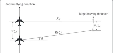
peaks decide the trajectory of the RMC during synthetic aperture time. To implement RMC fitting, Ri(η) which indicates the instantaneous slant range between antenna phase center (APC) and the scattering center should be well understood. As show in Fig. 1, Ri(η)can be formu-lated as:
Ri(η)=
R20i+Vri2(η−η0i)2, (3)
where theith scattering center has the nearest slant range R0iat the timeη0iand relative velocityVribetween APC and itself. Consider some scattering centers may be mov-ing target,Vri=V−vaimay not be the same as platform speed V (see Fig. 1). To simplify the further derivation, Ri(η)is approximated with Taylor’s series. In squint mode,
Fig. 1SAR raw data acquisition geometry on slant range plane
R0itanθ/Vribe the offset between zero doppler timeηoi and beam center timeζi, which yields:
ζi=η0i−ηci. (4)
Since we assume both the exposure time and the squint angle are moderate, the terms up to quadratic order in (5) are sufficient to model a RMC precisely.
Define a new coordinate:
in which the subscriptnrepresents discrete sampling and γ scales fast time 2Ri(ηn)/cto a similar scale of magni-tude of slow timeηn. Here,γ=PRI·fsis decided by range sampling frequencyfs and pulse repetition interval PRI. For convenience, we letϑ = c/2γ. Together with (5), the discrete version of theith scattering center’s RMC can be modeled as: parameterizes the RMC of an individual scattering cen-ter, is estimated scatter by scatter. Applying the estimated
μ, the backscattering envelopeσ can be extracted from range-compressed signal. Along with it, the geographical information R0 and η0 and the relative velocity Vr will be reconstructed. The process will be detailed in the next section.
3 M-RANSAC-based feature extraction algorithm
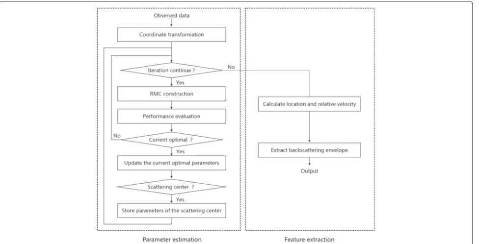
The proposed algorithm is an iterative method to esti-mate μ of different scattering centers through fitting their RMCs. Then, the estimated parameters will be used to realize feature extraction . As shown in Fig. 2, this algorithm consists of two major steps: parameter estima-tion and feature extracestima-tion.
In the step of parameter estimation, the observed data is extracted from the contour of the range-compressed signal. It is a mix set of “inliers” and “outliers”, indicating the trajectories of RMCs. The inliers can be explained by the parameter setμof current scattering center, while the outliers do not fit the model and may come from other scattering centers’ RMCs or noise.
To separate the inliers from the outliers and obtain the current optimal fitting RMC with parameterized repre-sentationμ, RMC construction and performance measure are implemented iteratively in this algorithm. The itera-tive procedure of M-RANSAC-based approach continues until the points within observed data set are classified according to their corresponding RMCs, thus scattering centers. Along with the classified points, the overall num-ber of scattering centersMand a set ofμcorresponding to different scattering centers are obtained.
Then, the step of feature extraction starts with these classified points and the estimated μ. The loca- tion and relative velocity of scattering centers can be directly reconstructed byμ. The backscattering scattering envelopes will be extracted from the range-compressed signal. Thus, feature extraction of M scattering centers are accomplished. The details of parameter estimation and feature extraction are summarized in the following subsections.
3.1 RMC construction with hypothetical inliers
Within a single iteration, a subset of observed data is randomly selected to construct a candidate RMC with the parametric representationμc. However, the observed data, which is directly extracted from the contour of the range-compressed signal, is sampled by sampling fre-quencyfsand pulse repetition frequency 1/PRI. Thus, the original coordinate of the observed datax=(x,y)T obvi-ously differs from the new coordinate ψ = (X,Y)T in (6). To locate the points of subset in the new coordinate system, a coordinate transformation should be processed first. The mapping relationship is expressed as:
Fig. 2Flowchart of M-RANSAC-based feature extraction algorithm
After coordinate transformation, the subset data in the new coordinate system is qualified for RMC construc-tion. Since the degree of freedom (DOF) of (7) is three, a subset withψ1,ψ2, andψ3is sufficient to calculate
corre-sponding model parameters.μcof this candidate RMC is therefore computed by:
Ac=
X12Y23−X23Y12 X23Y12∗ −Y12Y23∗
Bc=
X23Y12∗ −X12Y23∗ Y23Y12∗ −Y12Y23∗
Cc=X1−AcY12−BcY1
(11)
in which
Xij=Xi−Xj and Xij∗=Xi2−Xj2 (12)
The accurate construction mainly depends on the accu-racy of the selected points to solve (11). Only whenψ1,ψ2,
andψ3come from the same RMC, this constructedμccan be the parametric representation of a scattering center. However, the randomly chosen points might belong to dif-ferent RMCs or be just noise points. Therefore, to assess the performance of this constructed RMC, a measure needs to be established in the iterations.
3.2 Performance measure establishment based on quadratic orthogonal distance
In this subsection, a double-measure system is developed to evaluate the performance of a candidate RMC. To deal with the situation that selected points come from different
RMCs or are noise points, CFC, which denotes the num-ber of points in observed data set can be explained by the candidate RMC withμc, is introduced. Another measure, called FPI, is proposed to assure that a more precise RMC will be chosen when two candidate RMCs share the same CFC.
To judge whether a point can be explained by the candi-date RMC, quadratic orthogonal distance (QOD) between a point and a curve is developed. The qualification of a point is decided by its QOD to the RMC with a specific threshold value. Other than the least-squares distance, QOD is defined as the minimum connecting length from a point to the given curve, which is more precise in practical applications [21]. To obtain this distance, the geomet-ric feature of RMC is further analyzed. After coordinate transformation, RMC can be considered as a parabola with the vertex atψct=
C− B4A2,−2BA
. According to (7), the mathematical expression of RMC can be written as:
X−
C− B 2
4A
=A
Y+ B 2A
2
. (13)
As shown in Fig. 3,ψg is a point in the observed data. To calculate the QOD betweenψg and a candidate RMC parameterized with μc, ψp, which is the closest projec-tion ofψgon the RMC, should be located. Defineψg =
Xg,Yg
andψp=
Xp,Yp
. Sinceψplocates on the RMC, an equation can be obtained:
f1
Xp,Yp
Fig. 3Quadratic orthogonal distance to a curve
Moreover, the connecting line ofψgandψpis perpendic-ular to the tangent line of the RMC at the pointψp. This relationship can be formulated as:
dY
Rewriting the above equation, it yields:
f2
Combining (14) and (16) into a quartic equation will result in maximum four solutions. Generally, the solution with the minimum geometric distance to ψg is chosen as the optimal projection ψp. However, this numerical method is not stable. To optimize the calculation, Ahn [21] proposes a generalized Newton-Raphson method to locate the closest projection point. It is an efficient itera-tive method which converges quickly. Given the functions f1Xp,Ypandf2Xp,Yp, we define the derivative matrix D, the current approximate resultψk, and a more accu-rate approximationψk+1to computeψp. The process of iterations can be presented as:
Dψ= −f ψk
An initial valueψ0is given in Fig. 3, and its expression is:
Equation 17 starts its iteration with the initial valueψ0
and ends when|ψ|is no more than a given threshold. During the iterations, parameters related toψpin (18) are assigned with the value of the current iterative resultψk, and the final closest projectionψpis set to beψkwhen the iterations end. Therefore, we define the square Euclidean distance betweenψpandψgas the QOD ofψg:
rho= | ψg− ψp|2. (20)
When rho ofψg stays no more than the given thresh-old rho_thr, this point is regarded as an inlier, otherwise an outlier. The overall number of inliersN(μc)within the observed data is denominated as CFC. As shown in Fig. 4, this measure utilizes the number of inliers to define the fit-ting degree of the candidate RMC. To evaluate the degree of matching between the inliers and the candidate RMC, FPI is introduced as:
χ(μ)= − N
k=1
ε (rho_thr−rhok)·rhok. (21)
in which ε means unit step function. FPI, which is the negative overall QOD of inliers, is known as the accuracy of fitting. It works cooperatively with CFC to locate the optimal candidate RMC with the largest num-ber of inliers and best fitting precision. Conventional RANSAC-based algorithm [22] only considers CFC as measure without applying weighting for inliers’ QOD and the maximum likelihood estimation sample consensus (MLESAC)-based method [23] obtains the overall error with a computationally complicated process. They fail in either accuracy or efficiency. The double-measure sys-tem of CFC and FPI in this algorithm steps out of this dilemma and achieves a balance between precision and efficiency.
Fig. 4Construction fitness coefficient (the number of inliers for givenμk)
change from set to set. Based on the observed sets, 100 Monte-Carlo tests are conducted with iterative times 50, 100, 150 and 200. First, the average Euclidean norm of parameter setμ’s estimation error μˆversus iterative times are provided when the RMC is fitted by three differ-ent algorithms respectively. As shown in Fig. 5b, both the estimation accuracy and the convergence rate of MLESAC and M-RANSAC methods outperform those processed by RANSAC method. And, the estimation accuracy of the M-RANSAC method is surpassed by that of the MLESAC
method. However, the superiority of MLESAC’s perfor-mance costs heavy computational burden. In this paper, the computational times on a desktop PC (i5-3210M CPU at 2.5 GHz and DDR3 RAM at 8 GB) corresponding to iterative times are listed in Fig. 5c. According to this figure, we can tell the computational efficiency of MLESAC is obviously surpassed by those of the M-RANSAC and RANSAC methods. Therefore, to balance the accuracy and efficiency, the application of M-RANSAC algorithm may be the optimal choice for RMC fitting, and the
superior performance of this double-measure system is validated.
In the next subsection, M-RANSAC approach will inte-grate the measures and RMC construction into the itera-tive process of parameter estimation.
3.3 Iterative procedure of parameter estimation in M-RANSAC-based approach
The iterative process of proposed algorithm starts with a set of observed data D_set. It contains the points extracted from the contour of range compressed results and indicates the RMC trajectories of different scatter-ing centers. This set also inevitably contains many noise points introduced by undesired background information. M-RANSAC-based algorithm is proposed to classify the groups of points corresponding to different scattering centers, get rid of existing noise, and realize parameter estimation of these RMCs simultaneously. The pseu-docode of this process is displayed in Fig. 6. It consists of iterations of two levels: point-level iterations and scatter-level iterations. In the point-scatter-level iterations, a parametric RMC with optimal CFC and FPI is located to explain a scattering center. Then, the scatter-level iterations will lock all these RMCs in a range-compressed signal scatter by scatter.
Fig. 6The pseudocode of parameter estimation in M-RANSAC-based approach
To begin with, the minimum iterative times min, max-imum iterative times max, the threshold QOD to define an inlier rho_thr and the threshold number of inliers to confirm a scattering center N_thr should be preestab-lished. What is more, we should initialize maximum non-updating times m to infinite, the number of scattering center M to zero, and the iteration proceeding factor CONT to 1.
A point-level iteration starts with randomly selecting three points fromD_set to construct a candidate RMC. Theμcof this RMC is computed with (9) and (11). Then, according to subsection 3.2, the QOD between every point in theD_setand this candidate RMC are calculated and denoted by rho. The points whose rho stay no more than rho_thr are defined as inliers and stored in set(μc). Then, CFCN(μc)and FPIχ(μc)of this candidate RMC can be computed by (20) and (21).
This RMC can be regarded as the current optimal one in two cases. The CFCN(μc)exceeds that of the former optimal BestN, or the FPI χ(μc) goes over that of for-mer optimal Bestχ under the circumstance that N(μc) equalsBestN. When the conditions are satisfied and the current optimal is renewed, not onlyBestμ,BestN,Bestχ, and Bestset are updated in line with the values of cur-rent optimal RMC but also the maximum non-updating times m will be recalculated. The point-level iteration stops when iterative timesiterationexceed max or non-updating timesnon_updsurpassm. An additional mini-mum iteration times min is used to remain the stability.
In scatter-level iterations, a new scattering center will be confirmed when the output of the point-level itera-tionsBestNgoes beyondN_thr. At this time, the number of recovered scattering centersMis updated.Bestμand Bestset are stored in setμ(M) and set(M). The idea of CLEAN technique [24, 25] are taken, and the points in Bestset will be subtracted from D_set. Another point-level iterations will be processed to locate the next RMC. Oppositely, if the point-level iteration fails to locate a scattering center, the remaining points in observed data set are considered as noise points. Thus, the scatter-level iterations stop by setting CONT=0.
After the two-level iterations, the total number of scat-tering centersMis determined, the points of inliers are classified in set, and the parametric representationμ of scattering centers are estimated and saved insetμ. These data will help to realize feature extraction for dominant scattering centers of the targets in the next subsection.
relative velocity between the radar platform and scatter-ing center, indicates the possible along-track speed of the scatter. They can be reconstructed using the estimatedμi insetμ(i):
In broadside case, sinθ and tanθ equal zero. (22) degrades to a simpler formula:
R0i =ϑ
pr, azimuth beam pattern wa, and the phase informa-tion related to instantaneous slant range Ri are calcu-lated. By locating inliersset(i) in the range-compressed signal, the complex values along the RMC of scatter-ing center can be extracted. Accordscatter-ing to (2), we obtain the complex backscattering envelopeσi(η−ζi)by elim-inating the influence of the aforementioned compo-nents in the extracted complex values. The vector set
T1, T2,. . . TM
are calculated scatter by scatter. It is worth noting that, the process of M-RANSAC-based algorithm does not need the explicit parameters (e.g., platform velocity). However, for conventional meth-ods of feature extraction based on SAR image formation, the platform velocity works as a crucial parameter of realizing range cell migration correction (RCMC) and azimuth matched filtering. Thus, compared with the con-ventional approach, M-RANSAC-based algorithm can be utilized in a more flexible way. Moreover, the proposed algorithm extracts the features directly from a range-compressed signal. Without forming SAR image, we may realize target recognition and classification directly in a signal level rather than in an image level.
When platform velocity is known and SAR image is formed, the backscattering envelope extracted by the pro-posed algorithm may classify targets which are similar in the gray-level SAR image. Moreover, given the platform velocity and the relative velocity between radar platform
and the dominant scattering center, the along-track veloc-ity of target can be computed. Thus, even if SAR image is formed, this feature extraction algorithm may help us to better understand the target.
4 Trajectories separation based on STFRFT
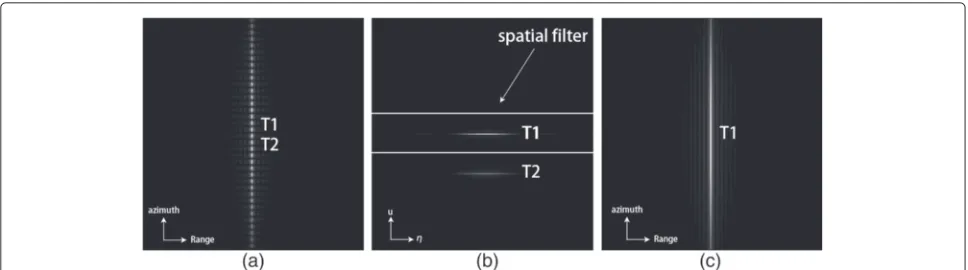
Sometimes, RMC of one scattering center may overlap that of the other. This phenomenon is called trajecto-ries overlapping in this paper. As shown in Fig. 7a, the trajectories of T1 and T2 are mixed after range com-pression (to clearly state the principle, the range curve are ignored under the low-resolution assumption). In this case, M-RANSAC-based algorithm may fail in extract-ing interested information of T1 and T2, respectively. To solve this problem, short-time fractional Fourier trans-form (STFRFT) is applied to separate the overlapped trajectories. With a spatial filtering using a rectangle win-dow, the trajectories of different scattering centers will be separated in time-fractional frequency domain. The fea-ture extraction can be successfully proceeded afterwards.
The phase component in (2) can be written as:
sφ(η)=
Here, Ka is considered as a constant. It is a reason-able assumption when the range span of processed data is moderate. fi, related to the beam center time ζi, dif-fers with the azimuth location of scattering center. Taking STFRFT of (24), it yields:
STFφ(η,u)=
Fig. 7Trajectories separation based on STFRFT.aOverlapped trajectories of T1 and T2.bMatched STFRFT and spatial filter of trajectories in selected range bin.cSeparated trajectory of T1
Kp(t,u)=
Based on the frequency shift property of STFRFT [20], (26) becomes:
Note that (30) is a matched STFRFT only when the second-order phase term is set to zero, thus,αis:
α=arc cot!2πKa·NaPRI2
"
(31)
where,PRIis the pulse repetition interval andNadenotes the length of azimuth sample. In the real application, NaPRI2 is used as the factor of coordinate transfor-mation in digitalized computation [26, 27]. Back to (29), the STFRFT of an individual scattering center is decided by STFKa(η,u). The matched STFRFT of (30)
will locate the spectrogram line of a scattering center parallel to η. For multiple scattering centers, the shift u = −2πfisinα along u axis in (29) separates their energy according to their different azimuth locations. As shown in Fig. 7b, a simple spatial filter using a rectan-gle window will separate the energy of one scattering center from the others. After inverse STFRFT, the tra-jectories of scattering centers with similar range posi-tion but different azimuth locaposi-tion are separated (e.g., Fig. 7c).
To realize trajectories separation in feature extaction, the STFRFT-based method is embedded in the afore-mentioned M-RANSAC-based approach. The processing steps can be summarized as follows:
1. Select the trajectory of an isolated scattering center and estimateKausing the points extracted from it.
2. Calculateαbased on (31).
3. Executeα-angle STFRFT for a range bin.
4. Implement spatial filtering using rectangle windows. 5. Realize trajectories separation with inverse STFRFT. 6. Repeat steps 3 to 5 until the last range bin is
processed.
7. For every sub-patch range compressed signal,
estimateM,setμ, andset using M-RANSAC
approach.
8. Use the estimatedM,setμ, andset to compute the vector set T1, T2,. . . TM
.
5 CRLB and RMSE of parameter estimation
The parameter estimation ofμlays the foundation for fea-ture extraction in this algorithm. In this section, Monte-Carlo tests are conducted to obtain the root mean squared errors (RMSEs) of the estimates. To evaluate the accuracy of estimation, these RMSEs of estimators compared their theoretical minimal errors, named Cramér-Rao lower bound (CRLB). We start this section with computing the CRLBs according to observation.
The observation can be derived from (2) and (7):
Here, ω0(n) denotes a complex white noise with zero
mean and the variance ofσ0. The estimator vectorφe = [Aˆ,Bˆ,Cˆ] contains three parameters waiting to be esti-mated.
According to [28], the Fisher information matrix of (32) can be calculated using the expression:
$
The computation of its inverse is complicated and tedious, we omit the procedures of derivation and directly give the result:
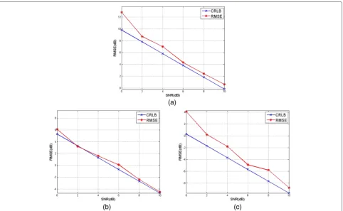
where the is the average amplitude of backscat-tering envelope σ{n·PRI} and azimuth beam estimated parameters are the diagonal elements of inverse matrix. Thus, the CRLBs of Aˆ, Bˆ, and Cˆ are equal to
Then, 100 Monte-Carlo tests are conducted when signal-to-noise ratio (SNR) is 0, 2, 4, 6, 8, and 10 dB, respectively. The experiments utilize the SAR simulation parameters listed in Table 1. To better exhibit the results, both RMSEs and CRLBs of the estimated parameters are expressed in decibels. As shown in Fig. 8, the RMSEs of the estimated values stay close to their CRLBs. Since CRLB is the theoretical lowest estimation error, we can conclude that the parameter estimation based on the pro-posed algorithm is accurate and effective. The precisely
Table 1System parameter of simulation and real data
Parameter Simulation test Real data experiment Squint angle 0◦ −1.584◦
Signal bandwidth 150 MHz 30.111 MHz Sample frequency 200 MHz 32.317 MHz Pulse duration 5.12μs 41.74μs
PRI 1.7 ms 0.7956 ms
Platform velocity 153.3 m/s 7062 m/s Range to scene center 7500 m 998263 m
estimated parameters guarantee the subsequent process of feature extraction.
6 Experimental results
To validate the performance of this algorithm, a series of experiments, named performance test, simulation test, and real data test, respectively, are presented in this section. In the performance test, we generate raw data of a single target when the broadside airborne SAR system operates. This raw data is added with various Gaussian white noise and then taken as the input of M-RANSAC algorithm to estimate the location and veloc-ity of dominant scattering center. RMSE of the esti-mated parameters are listed corresponding to different input SNR and iterative times. Then, the scenario of multiple targets is considered in the simulation test. In the illuminated scene, three targets with different backscattering envelopes and along-track velocities are introduced. The features of dominant scattering centers are extracted from the generated data by M-RANSAC-based algorithm and compared with the theoretical ones. In addition, the potential usage of these extracted fea-tures in target recognition and classification are fully considered. In the end, the real data of RADARSAT-1 are processed to validate the performance of the pro-posed algorithm when the trajectories of targets are over-lapped. The features of the dominant scattering centers, including locations, relative velocities, and backscatter-ing envelopes, are extracted usbackscatter-ing both STFRFT-based trajectories separation and M-RANSAC-based feature extraction method. To verify the effectiveness of feature extraction, the reconstructed locations and velocities are compared with those obtained using conventional meth-ods. To confirm the potential usage of these extracted fea-tures in target classification, the backscattering envelopes are used to further interpret the ships in English Bay which is located in the city of Vancouver, Canada (see Fig. 13a).
6.1 Performance test
In this subsection, raw data of a single target are sim-ulated to evaluate the estimation accuracy. This target is a stationary one with the geographical location R0 =
7500 m andη0=0.8717 s. In the simulation, the system
parameters are listed in the middle column of Table 1 and beam width in azimuth dimension is set to be 0.059 rad. The generated raw data are added with Gaussian white noise when the input SNR= −10,−5, 0, 5, and 10 dB. For each input SNR, we generate 150 sets of random Gaus-sian noise; thus, in total, 750 sets of observed raw data are obtained.
Fig. 8RMSEs of parameter estimation and their CRLBs.aRMSE and CRLB of A.bRMSE and CRLB of B.cRMSE and CRLB of C
ϑ in (10) is set to be 450. The threshold of quadratic orthogonal distance rho_thr is 0.003 and the threshold number of inliers N_thr is 0.85Na. The overall iterative times are set to be a fixed numberTiter =50, 100, 150,
and 500. After estimatingμfor theMdominant scattering centers and classifying inliers inset, the geographical loca-tions and velocity information are reconstructed based on (23). For each input SNR, 150 sets of observed raw data will output 150 sets of Rˆ0, ηˆ0, Vˆr
. Compared with the theoretical ones, RMSE of {R0, η0, Vr} correspond-ing to different input SNR and iterative times are obtained and shown in Fig. 9b–d. According to this figure, several conclusions can be made:
(1) The estimation errors of location and relative velocity are quite limited especially when input SNR is 5 and 10 dB. Thus, We can expect a high
estimation accuracy in a high-SNR case.
(2) The estimation accuracy may decrease along with the input SNR. The reasonable explanation is that a higher-level noise will impact the precision of inliers in a larger degree and thus decrease the estimation accuracy. In the performance test, this phenomenon becomes obvious when the low-SNR data is
implemented.
(3) The estimation accuracy will be continuously enhanced with the increasing of iterative times until it converges. When input SNR is high, the estimation error converges fast. We can expect a high-precision output with a small number of iterative numbers. However, under low-SNR scenario, the estimation error converges slowly. max can be considerably increased to obtain relatively high-accuracy estimators. Unfortunately, there exists no SNR-related closed-form expression of max. The initial parameter max is an empirical parameter in this paper.
6.2 Simulation test
Fig. 9Performance test.aTime-domain range compressed signal with different input SNR (range-compressed azimuth-time domain).bRMSE ofR0. cRMSE ofη0.dRMSE ofVr
are shown in Fig. 10c. In the illuminated scene, we have two azimuth invariant point targets: T1 and T2. The amplitude and phase of their theoretical backscattering envelopes are presented in Fig. 11a, b, respectively. T1 is set to be “brighter” than T2, which means it has a rela-tively higher backscattering coefficient or a larger radar cross section (RCS) [29]. We also have an azimuth variant point target T3, the maximum backscattering envelope of which stays lower than both T1 and T2 (see Fig. 11a).
Different from T1 and T2, T3 has an inconstant phase envelope during the synthetic aperture time (see Fig. 11b). In the simulation test, these targets are customized with the size of 2 m in range by 1 m in azimuth, and their geo-graphical locations are shown in the columnsR0andη0 of Table 2. Moreover, both T1 and T3 are stationary tar-gets while T2 is a moving target with a 5.5 m/s along-track velocity. The relative speed between radar platform and targets are listed in the columnVrof Table 2.
Fig. 11Backscattering envelopes of targets.aTheoretical backscattering amplitude envelopes of targets and the extracted ones of dominant scattering centers.bBackscattering phase envelopes of targets
Using the SAR simulation parameters in Table 1, we generate the raw data of these three targets when SNR is 5 dB and beam width in azimuth dimension is 0.0785 rad. In this case, the Doppler spectrum of the range-compressed signal wraps around azimuth frequency as a result of ambiguity (see Fig. 12a). It may degrade the effectiveness of feature extraction algorithm starting with spectrum. To validate this assumption, a FFT-based time-frequency approach [8] and a complex spectral estimation algorithm called APES [16] are used to extract the spec-tral envelope of T3 respectively. As shown in Fig. 12b, the extracted results differ from the real data due to the impact of ambiguity. Thus, the proposed M-RANSAC-based feature extraction algorithm, which establishes itself as an ambiguity-free approach, is required in this case. The M-RANSAC-based algorithm starts with time-domain range compressed signal (see Fig. 12c). Its initial parameters are carefully designed. The scale factor ϑ in (10) is set to be 450. The lower bound of iterative times min is 30 and the upper bound max is 200, the thresh-old of quadratic orthogonal distance rho_thr is 0.003, and the threshold number of inliers N_thr is 0.85Na. After estimatingμ for theMdominant scattering centers and classifying inliers in set, the geographical locations and velocity information are reconstructed based on (23). As
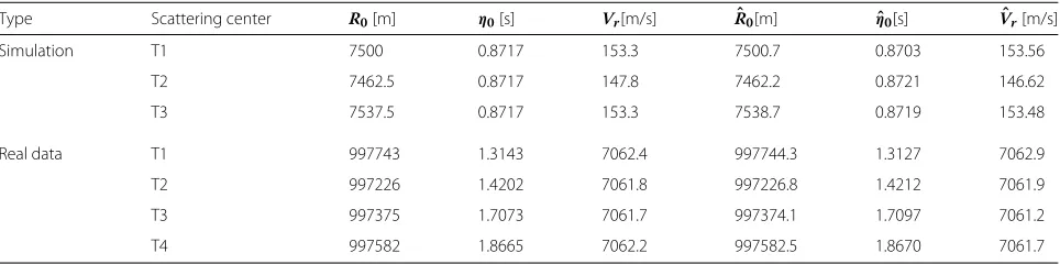
shown in the columnsRˆ0,ηˆ0, andVrˆ of Table 2, the esti-mated errors are quite limited. Meanwhile, the backscat-tering envelopes are extracted and normalized. In Fig.11a, the extracted backscattering amplitude envelopes of dom-inant scattering centers match the theoretical ones of the corresponding targets.
Without knowing the explicit knowledge of platform velocity and forming a SAR image, the extracted backscat-tering envelopes can label T1 and T2 as azimuth invariant targets and T3 as an azimuth variant target. Thus, a rough target classification can be achieved.Rˆ0 andηˆ0 present the geographical locations of dominant scattering centers. To visualize the extracted information, we mapRˆ0andηˆ0 of scattering centers into image domain. The amplitudes of them are obtained by averaging their backscattering envelopes. As shown in Fig. 12d, the image is free from the impact of sidelobes. Realizing the target classification and location, M-RANSAC-based algorithm help us to comprehend the targets without forming a SAR image.
When the explicit platform velocity is given, SAR image (see Fig. 12f) can be formed by chirp-scaling algorithm [30, 31]. Figure 12e presents the imaging result with eight times interpolation. In this image, T1 is well-focused while T2 and T3 are defocused. From the perspective of SAR image, T2 and T3 may be mistakenly classified
Table 2Original and estimated parameters in both simulation test and real data test
Type Scattering center R0[m] η0[s] Vr[m/s] Rˆ0[m] η0ˆ [s] Vˆr[m/s]
Simulation T1 7500 0.8717 153.3 7500.7 0.8703 153.56
T2 7462.5 0.8717 147.8 7462.2 0.8721 146.62
T3 7537.5 0.8717 153.3 7538.7 0.8719 153.48
Real data T1 997743 1.3143 7062.4 997744.3 1.3127 7062.9
T2 997226 1.4202 7061.8 997226.8 1.4212 7061.9
T3 997375 1.7073 7061.7 997374.1 1.7097 7061.2
Fig. 12Simulation test.aDoppler spectrum of a range-compressed signal (range-compressed Doppler domain).bExtracted spectral envelopes of T3 using FFT and APES.cTime-domain range-compressed signal (range-compressed azimuth-time domain).dSAR image formed by mapping the extracted feature.eSAR image with eight times interpolation formed by chirp-scaling algorithm.fSAR image formed by chirp-scaling algorithm
into the same type. However, defocus only indicates the mismatch of azimuth matched filter. It may result from either the along-track motion (T2) or the invariant azimuth envelope (T3). Since the two cases are hardly dis-tinguished directly from SAR image, the importance of feature extraction is proved. The extracted envelopes of dominant scattering centers in Fig. 11a clearly reveals the backscattering feature of targets. Thus, we can label T1 and T2 as azimuth invariant targets and T3 an azimuth variant one. The backscattering envelope of target’s dom-inant scattering center can be complementary to the SAR image in the application of target classification. Moreover, given the explicit platform velocity, we confirm T2 as a moving target according to columnVrˆ of Table 2.
6.3 Real data test
In this subsection, RADARSAT-1 raw data included in the CD of [19] is applied in feature extraction. The key sys-tem parameters are listed in Table 1. As shown in Fig. 13a, the SAR image of English Bay is formed using the chirp-scaling algorithm. Then, the region of four ships, marked with a white rectangle, are truncated from this SAR image. This patch of complex image is converted to a range-compressed signal (use inverse chirp-scaling algorithm and range matched filter).
Fig. 13Experimental results based on RADARSAT-1 data.aSAR image formed by chirp-scaling algorithm.bTrajectories of RMCs of ships in time-domain range compressed signal.cThe result of trajectories separation based on STFRFT.dExtracted backscattering amplitude envelopes of dominant scattering centers
estimated using the dominant scattering center of iso-lated ship T1. Then,αis computed by (31). Usingα-angle STFRFT and spatial filtering, the energy of T3 are sep-arated from the whole range-compressed signal. After inverse STFRFT, two sub-patch results are obtained (see Fig. 13c).
The M-RASNAC-based feature extraction algorithm starts with the range-compressed signal in Fig. 13c. The scale factorϑ =5800 in (10), the lower bound of itera-tive times min= 30, and the upper bound max= 300, the threshold of quadratic orthogonal distance rho_thr= 0.0016, and the threshold number of inliersN_thr=0.85· Na. After estimatingμ for the dominant scattering cen-ters of each ship, the geographical locations and velocity information are reconstructed based on (22) (see columns
ˆ
R0, ηˆ0, and Vrˆ of Table 2). To verify the performance of parameters construction, we define the dominant scattering center of a ship as the point with maximum
amplitude in SAR image. Their geographical locations are listed in columnsR0andη0of Table 2. The micro along-track velocity of dominant scattering centers are esti-mated using fractional Fourier transform (FRFT)-based method introduced in [32]. The relative velocity between radar platform and these scattering centers are then listed in columnVrˆ of Table 2. Since two groups of data are in good agreements, the reconstructed errors are quite limited.
7 Conclusions
An M-RANSAC and STFRFT-based technique is intro-duced to extract feature of SAR dominant scattering centers in this paper. Starting with the time-domain range-compressed signal, this algorithm provides an ambiguity-free signal-level approach. Meanwhile, this algorithm requires no explicit knowledge of platform velocity. It can conduct feature extraction without forming a SAR image. Within the extracted features, the backscat-tering envelope is promising to classify the target type in signal level, the geographical location indicates the target position relative to SAR platform, and the relative velocity denotes the along-track motion of illuminated target.
Experiments are conducted to illustrate the perfor-mance of this algorithm. In the tests, the estimation errors of location and relative velocity are quite limited when SNR is relatively high. The normalized extracted backscattering envelopes express their theoretical ones well. Moreover, these extracted features validate their usage in target recognition and classification. Without forming a SAR image, these extracted features will help us roughly understand and classify the illuminated targets. When SAR image is formed by conventional methods, the extracted backscattering envelopes can be complemen-tary to SAR image in the application of target recognition and classification.
Competing interests
The authors declare that they have no competing interests.
Acknowledgements
This work has been supported by key project of the National Natural Science Foundation (NNSF) of China (nos.61132005). The authors also want to express gratitude to editors and anonymous reviewers who give the helpful comments and suggestions to his paper.
Received: 2 July 2015 Accepted: 31 March 2016
References
1. DE Dudgeon, RT Lacoss, An overview of automatic target recognition. Lincoln Lab J.6(1), 3–10 (1993)
2. GJ Owirka, SM Verbout, LM Novak, inAeroSense’99. Template-based SAR ATR performance using different image enhancement techniques (SPIE, Bellingham WA 98227-0010 USA, 1999), pp. 302–319. International Society for Optics and Photonics
3. Z Jianxiong, S Zhiguang, C Xiao, F Qiang, Automatic target recognition of SAR images based on global scattering center model. IEEE Trans Geosci Remote Sens.49(10), 3713–3729 (2011)
4. Y Chen, E Blasch, H Chen, T Qian, G Chen, inSPIE Defense and Security Symposium. Experimental feature-based SAR ATR performance evaluation under different operational conditions (SPIE, Bellingham WA 98227-0010 USA, 2008), pp. 69680–69680. International Society for Optics and Photonics
5. Y Huang, J Pei, J Yang, T Wang, H Yang, B Wang, Kernel generalized neighbor discriminant embedding for SAR automatic target recognition. EURASIP J Adv Signal Process.2014(1), 1–6 (2014)
6. JB Keller, Geometrical theory of diffraction. JOSA.52(2), 116–130 (1962) 7. LC Potter, RL Moses, Attributed scattering centers for SAR ATR. IEEE Trans
Image Process.6(1), 79–91 (1997)
8. M Spigai, C Tison, J-C Souyris, Time-frequency analysis in high-resolution SAR imagery. IEEE Trans Geosci Remote Sens.49(7), 2699–2711 (2011)
9. VC Chen, H Ling,Time-Frequency Transforms for Radar Imaging and Signal Analysis. (Artech House, Norwood, 2001)
10. J-P Ovarlez, L Vignaud, J-C Castelli, M Tria, M Benidir, Analysis of SAR images by multidimensional wavelet transform. IEE Proc Radar Sonar Navig.150(4), 234–241 (2003)
11. G Lisini, C Tison, F Tupin, P Gamba, Feature fusion to improve road network extraction in high-resolution SAR images. IEEE Geosci Remote Sens Lett.3(2), 217–221 (2006)
12. Z-S Liu, J Li, inRadar, Sonar and Navigation, IEE Proceedings-. Feature extraction of SAR targets consisting of trihedral and dihedral corner reflectors, vol. 145 (IET, Michael Faraday House, Six Hills Way Stevenage, Herts, SG1 2AY, UK, 1998), pp. 161–172
13. Z Bi, J Li, Z-S Liu, Super resolution SAR imaging via parametric spectral estimation methods. IEEE Trans Aerosp Electron Syst.35(1), 267–281 (1999)
14. J Li, P Stoica, Efficient mixed-spectrum estimation with applications to target feature extraction. IEEE Trans Signal Process.44(2), 281–295 (1996) 15. EG Larsson, G Liu, P Stoica, J Li, High-resolution SAR imaging with angular
diversity. IEEE Trans Aerosp Electron Syst.37(4), 1359–1372 (2001) 16. J Li, P Stoica, An adaptive filtering approach to spectral estimation and
SAR imaging. IEEE Trans Signal Process.44(6), 1469–1484 (1996) 17. SR DeGraaf, Sidelobe reduction via adaptive FIR filtering in SAR imagery.
IEEE Trans. Image Process.3(3), 292–301 (1994)
18. R Wu, J Li, Z Bi, P Stoica, SAR image formation via semiparametric spectral estimation. IEEE Trans Aerosp Electron Syst.35(4), 1318–1333 (1999) 19. IG Cumming, FH-c Wong,Digital Processing of Synthetic Aperture Radar
Data: Algorithms and Implementation. (Artech House, Norwood, 2005) 20. R Tao, Y-L Li, Y Wang, Short-time fractional Fourier transform and its
applications. IEEE Trans Signal Process.58(5), 2568–2580 (2010) 21. SJ Ahn, W Rauh, H-J Warnecke, Least-squares orthogonal distances fitting
of circle, sphere, ellipse, hyperbola, and parabola. Pattern Recogn.34(12), 2283–2303 (2001)
22. YC Cheng, SC Lee, A new method for quadratic curve detection using K-RANSAC with acceleration techniques. Pattern Recogn.28(5), 663–682 (1995)
23. PH Torr, A Zisserman, MLESAC: a new robust estimator with application to estimating image geometry. Comput Vis Image Underst.78(1), 138–156 (2000)
24. J Tsao, BD Steinberg, Reduction of sidelobe and speckle artifacts in microwave imaging: the CLEAN technique. IEEE Trans. Antennas Propag.
36(4), 543–556 (1988)
25. H Deng, Effective CLEAN algorithms for performance-enhanced detection of binary coding radar signals. IEEE Trans Signal Process.52(1), 72–78 (2004)
26. HM Ozaktas, O Arikan, MA Kutay, G Bozdagi, Digital computation of the fractional Fourier transform. IEEE Trans. Signal Process.44(9), 2141–2150 (1996)
27. S Chiu, Application of fractional fourier transform to moving target indication via along-track interferometry. EURASIP J Appl Signal Process.
2005, 3293–3303 (2005)
28. TA Schonhoff, AA Giordano,Detection and Estimation Theory and Its Applications. (Pearson/Prentice Hall, New Jersey, 2006)
29. EF Knott,Radar Cross Section Measurements. (SciTech Publishing, Raleigh, 2006)
30. RK Raney, H Runge, R Bamler, IG Cumming, FH Wong, Precision SAR processing using chirp scaling. IEEE Trans Geosci Remote Sens.32(4), 786–799 (1994)
31. A Moreira, J Mittermayer, R Scheiber, Extended chirp scaling algorithm for air- and spaceborne SAR data processing in stripmap and ScanSAR imaging modes. IEEE Trans Geosci Remote Sens.34(5), 1123–1136 (1996) 32. J Yang, C Liu, Y Wang, Detection and imaging of ground moving targets