R E S E A R C H
Open Access
A recursive kinematic random forest and
alpha beta filter classifier for 2D radar tracks
Lars W. Jochumsen
1,2*, Jan Østergaard
2, Søren H. Jensen
2, Carmine Clemente
3and Morten Ø. Pedersen
1Abstract
In this work, we show that by using a recursive random forest together with an alpha beta filter classifier, it is possible to classify radar tracks from the tracks’ kinematic data. The kinematic data is from a 2D scanning radar without Doppler or height information. We use random forest as this classifier implicitly handles the uncertainty in the position
measurements. As stationary targets can have an apparently high speed because of the measurement uncertainty, we use an alpha beta filter classifier to classify stationary targets from moving targets. We show an overall classification rate from simulated data at 82.6 % and from real-world data at 79.7 %. Additional to the confusion matrix, we also show recordings of real-world data.
Keywords: Radar, Classification, Random forest, Alpha beta filter, Kinematic
1 Introduction
The increasing demand for protection and surveillance of the coastal areas requires modern coastal surveil-lance radars. These radars are designed such that small objects can be detected. Therefore, there is an increasing amount of information for the radar observer. Moreover, the number of false and unwanted objects increases as the demand for seeing small objects makes the radar more sensitive. Generally, the false objects can be avoided by using a reliable tracker. However, the tracker does not exclude unwanted objects. The difference between false and unwanted objects is that false objects do not originate from true objects but are mainly noise objects, whereas the unwanted objects originate from true objects but are unwanted in the surveillance image. These objects depend on the purpose of the radar; however, for coastal surveil-lance radars, the unwanted objects are normally birds, wakes from large ships, etc.
It has been shown in [1] that it is possible to classify tracks by using a recursive classifier where a Gaussian mixture model (GMM) is used to model the probabil-ity distribution function (PDF) of the target’s kinematic behavior. However the classifier does not handle the
*Correspondence: [email protected] 1Terma A/S, Hovmarken 4, Lystrup, Denmark
2Department of Electronic Systems, Aalborg University, Fredrik Bajers Vej 7b, Aalborg, Denmark
Full list of author information is available at the end of the article
uncertainty in the measurements from the radar. In [2], the position uncertainty is used as an input to the classi-fier. The classifier also use a GMM to model the PDF of the kinematic behavior of the target. The problem with this is that it is very computationally expensive. To obtain an easier way to handle uncertainty, joint target tracking and classification can be used, as shown in [3–5]. The problem with joint target tracking and classification is that it is dif-ficult to achieve a high degree of freedom in the filters to separate the classes. For example, a car driving 130 km/h on the highway is not likely to accelerate but more likely to decelerate. This is very hard to model with a tracking filter. A particle filter can be used, but this is computation-ally expensive. In [6], the authors are describing a method to classify trucks and cars from GPS measurements. The classifier consists of a support vector machine (SVM), and the features are primarily acceleration and deceleration. The classifier is non-recursive, which means that the com-plete length of the tracks is required. The measurements from a GPS device is generally more accurate than the position measurements from a radar. In [7], a decision tree is used for a recursive classification of four different target classes. The data are from a radar with height information. The decision tree has the advantage that it in some way implicitly handles the uncertainty, that is, features that do not separate the classes will not be used as much as fea-tures separating the classes. The disadvantage is that the classifier has a high variance of the classification results. In
[8], the random forest classifier is introduced. The random forest is a bagging classifier [9] where multiple decision trees are used to reduce the variance of the classification results. For this reason, random forest is selected in this work.
In this work, we introduce a classifier which uses posi-tion measurements to classify radar tracks from a 2D scanning radar. The classifier consists of an alpha beta fil-ter [10] and a random forest classifier. The alpha beta filfil-ter is classifying stationary or moving targets, and the random forest classifies moving targets. The classifier is recur-sive such that the classification results are being updated for each scan of the radar. The classifier performance is shown by using simulated track data and real-world radar data.
In Section 2.1, we will introduce the random forest clas-sifier by describing the training of a decision tree and then explain how this tree is used in the random forest. In Section 2.2, we will explain how we utilize the prob-ability estimates from the random forest in a recursive framework. In Section 2.3, we introduce an alpha beta fil-ter classifier, which classifies targets as either stationary or moving. This is introduced because stationary targets can have high speeds because they fluctuate in the position because of measurement uncertainty or the main scatter points are moving, i.e., wind turbine. In Section 2.4, we combine the random forest and the alpha beta filter as our proposed classifier. In Section 2.5, we describe which fea-tures we use in the random forest. The simulation study is shown in Section 3, and in Section 4, the real-world results are shown. We discuss the results in Section 5 and conclude the work in Section 6.
2 Method
When using a random forest, a feature vector is needed. We define our feature vector as a set of kinematic and geographic features. The feature vector is derived from the radar position measurements. We define this set of position measurements as
{Zn}k= {Zn· · ·Zn−k}, (1) whereZn=[xn,yn]T,xandyis the position in a Cartesian coordinate system with the origin at the location of the radar,nis the measurement number index, andkis the set size.
2.1 Random forest
In this section, we introduce the random forest classifier [8, 11]. The random forest is a bagging algorithm, which means that the random forest consists of a number of weak classifiers [12], which has zero bias but high vari-ance of the true value. The weak classifiers are decision trees [9]. We start this section by describing how to grow a decision tree and then move on to the random forest.
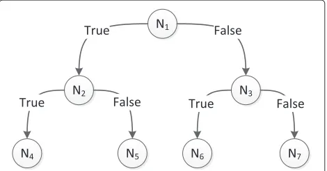
A decision tree consists of a number of nodes, e.g., (N1· · ·N3) and a number of leafs, e.g., (N4· · ·N7). This is shown in Fig. 1. A node is defined by more than one class existing in the node data, whereas a leaf has only one class. In every node, a decision must be made such that we go either left or right in the tree. The decision must always be true or false. A leaf is defined as a node where all of the data in the node consists of only one class; therefore, no more splits are required.
To train the tree, we start with a feature vectorFof size
Ns×DwhereNs is the number of samples andDis the number of features, i.e., dimensions in the feature vector. We now want to split the data such that we make the best separation of the classes by choosing the best feature and feature value. To do this, we need to find the best feature to split on and the best value to split at. To explain the algorithm, we assume that there are only two classes so it forms a binary classification problem and that the values of the feature belong to a finite sample space. This is done to make the explanation easier.
We start by assuming that a split already has been made and we want to evaluate how good the split is. For this, we use a normalized entropy measure to do that [12]. An alternative to the normalized entropy is the more common Gini index [13]; however, for this work, the normalized entropy has shown better results. We define the set of samples in the parent node ass1and the number of sam-ples in the set as|s1|. Similarly, we define the set of samples in the children ass2ands3and the number of samples as |s2|and|s3|. Further, we index the samples belonging to classby the superscriptsuch ass1, where∈ {1, 2}. We can calculate the empirical entropy for the children as
H(si)= −P
Fig. 1An example of a decision tree whereN1toN3are nodes where
into account how many samples there are in each child, we
We can now calculate the information gain from the split as
From (4), we now have a measure for how good a split is and now able to optimize each split of the data such that we choose the best feature to split on and the best value of the feature. We split the data and continue to split the data until all data in a node is of the same class, i.e., the node becomes a leaf. To prevent overfitting, a decision tree must be prone. However, an advantage of using ran-dom forest is that it is not necessary to prune the decision trees. The random forest is a bagging classifier [9]. This means that the random forest consists of a number of trees
Ntwhere each tree is trained with a random part of the samples and a random part of the features, that is, we draw a random subset of the training data and select a random subset of the features. We then train each tree with these random subsets, and we assume that the trees are statisti-cally independent of each other. A decision tree classifies the data by following a path through each node. The path is decided by the feature and feature value that made the best split in the training. The data which must be classified follow the path until a leaf is met. The leaf has a unique class, and the data is classified as this class. The classifica-tion of the data is a majority vote of the result from each of the individual decision trees, that is, each tree is a unique classifier which classifies the individual data.
In general, the random forest is not a probabilistic clas-sifier but a majority vote between each of the trees. How-ever, by counting the votes for each class and normalizing with the total number of trees, an empirical probability can be achieved.
ˆ
P(ci|{Zn}k)=ψi/Nt, (5)
whereψiis the the number of votes for classi.
In the next section, we explain how we obtained (5) from the random forest to achieve a recursive update of the probability for the class given all the measurements.
2.2 Recursive update of the random forest probability
The empirical probabilities obtained from the random for-est classifier are obtained as the fraction of the number of trees which predicts ci divided by the total number of trees. By this definition, the resolution of the prob-ability estimates is given by the number of trees in the
random forest. To prevent that a class is assigned a zero probability, we modify it in the following way:
P(ci|{Zn}k)=
ˆ
P(ci|{Zn}k)(1−2/Nt)+1/Nt
γ , (6)
where γ is a normalization constant such that
iP(ci|{Zn}k)=1. By this formula, the probability never reaches zero for any of the classes.
Based upon the above, we have the probability for the class given the current set of featuresP(ci|{Zn}k). How-ever, we want the probability given all measurements, that is P(ci|{Zn}), where {Zn} = {Zn}n. We have, however, not been able to find a simple way to recursively update
P(ci|{Zn})based on the previousP(ci|{Zn−1})and which works for alln. Instead, we propose the following recur-sive functionf(ci|{Zn}), which is everywhere non-negative and sums to one. Thus,f(ci|{Zn})can be considered to be a probability mass function (PMF), which we will use as an approximation for the trueP(ci|{Zn}). In particular, we and where φn is the normalization constant such that
cif({Zn}k = 1. The introduction of the weighting by
wis inspired by the weighted Bayesian classifier used in [14]. In particular, we choosew = 1/ksince the features of the random forest are given by a set of measurements where only one out ofk measurements is substituted at each update.
In the next section, we describe our alpha beta tracking filter. This filter is used to classify if a target is non-moving or moving. The reason for applying such a filter is to clas-sify stationary targets, which have a high apparent speed due to measurement uncertainties.
2.3 Alpha beta filter
The alpha beta filter is a simple tracking filter [15]. By using the alpha beta filter, we assume that we can describe the target movements with a first-order Markov chain. We have the state vectorXn =[xˆ,ˆy]T and the measurement
Zn. The alpha beta filter is trying to predictZngiven the speedVn−1at timen−1 and the stateXn−1as
Xn−=Xn+−1+τVn+−1, (8)
whereτ is the time betweenZn−1andZnand the super-script−is the prediction before the measurement is used and the superscript+ is after the measurement is used. The filter assumes the speed is constant betweennand
n−1, that isVn=Vn−1. The error can be calculated as
and with the residual, we update the estimate of theVn−
whereαandβare the constants in the alpha beta filter. To calculate the probability forZngivenXn−,α, andβ, we use
wherenis the covariance of the position and the sub-scriptαβ is to emphasize that this is the probability for the alpha beta filter. The purpose of the alpha beta filter is to separate non-moving targets, i.e., stationary targets from moving targets. We therefore define two filters: a stationary filter with the parameters α = 0.1 and β = 0.0, which allows the position part of the state to move slightly but forces the speed to be constant at zero. The possibility for a slight movement of the state is because of the possibility for false-starting measurements. As the parametersα andβ are given of the classcs, we use the notation Pαβ(Zn|Xn−cs). Likewise, we define the moving alpha beta filter as Pαβ(Zn|cm,Xn−) with the parameters
α = 1.0 and β = 1.0, i.e., we hold the speed constant from update to update but allow both the movement and the speed to change with the measured change. If we know{Zn−1}which is the set measurement up ton−1 and α and β, we can calculate Xn− and we can there-fore writePαβ(Zn|ci,{Zn−1})instead ofPαβ(Zn|ci,Xn−). For this work, we want the alpha beta filter to classify if the target is stationary or non-stationary, and we therefore recursively update the probability of the alpha beta filter.
Pαβ(ci|{Zn})=
Pαβ(Zn|ci,{Zn−1})Pαβ(ci|{Zn−1})
Pαβ(Zn|{Zn−1})
.
(12)
To reduce the computational complexity, we assume that the positions are controlled by a first-order Markov chain, i.e.,Zn↔Zn−1↔ {Zn−2},∀n.1
Pαβ(ci|{Zn})=
Pαβ(Zn|ci,Zn−1)Pαβ(ci|{Zn−1})
Pαβ(Zn|Zn−1)
, (13)
In the next section, we describe how we combine the random forest classifier and the alpha beta filter classifier such that a classifier, which is a combination of the two classifiers, is created.
2.4 Combining the alpha beta filter with random forest
In our work, we let the alpha beta filter classify if the target is stationary or non-stationary, i.e., the alpha beta filter has
two classes. The random forest has a stationary class and multiple non-stationary classes. We define for the random forestc0 to be the stationary class and c1···nC to be the moving classes, wherenC is the total number of classes. For the alpha beta filter, we have the two classes ascsand
cmfor stationary and non-stationary classes, respectively. We want the alpha beta filter classifier to have a larger weight on the classification result of stationary vs. mov-ing than the random forest. We therefore use the recursive updated probability from (13). We do this as described in (14) and (15). including the alpha beta filter in this manner, we ensure that the alpha beta filter classifies if a target is station-ary while the alpha beta filter classifier does not have influence on the different moving classes.
In the next section, we will describe the features we use for the random forest feature vector, and we will also describe how these are derived from the position. We only utilize position-dependent features such as speed and acceleration.
2.5 Features
For the feature vector, we draw inspiration from [16] for some of the features. In this work, we set the number of position measurements k in (1) to 10. The number of measurements used in the feature vector is a com-promise between the time it takes to get the number of measurements required for a full feature vector and the amount of information contained in the feature vector. Larger k requires more measurements, i.e., more time before a classification result is made, whereas for smaller
k, the first classification result comes earlier albeit with a greater uncertainty due to the smaller amount of avail-able information. The features and their descriptions can be seen in Table 1. Remember that we defined{Zn}kto be
Table 1The feature vector used. The number of measurement has been chosen to bek=10
Feature Feature description
std(i) Empirical standard deviation of sample-to-sample distances
v1
. .
. 2-point speed estimate
vk
mean(vi) Empirical mean of the speed
std(vi) Empirical standard deviation of the speed
a1
. .
. 2-point acceleration estimate
ak−1
mean(ai) Empirical mean of the acceleration
std(ai) Empirical standard deviation of the acceleration mean(a⊥i ) Empirical mean of the normal acceleration
std(a⊥i ) Empirical standard deviation of the normal acceleration |zk−z0| Total distance moved
mean(di) Empirical mean of the distance to coast line
observed at timeti. We start by calculating the vectorial distance between the measurements as
δi=Zi−Zi−1, (17) with the scalar distance given by
i= |Zi−Zi−1|, (18) and the time difference between the measurements as
τi=ti−ti−1. (19) The 2-point velocity estimate is
vi= τi i
, (20)
for 1≤i<k, and the 3-point acceleration estimate is
ai=
2(vi+1−vi)
τi+1+τi−1
, (21)
for 1≤i < (k−1). The normal accelerationa⊥i is given by the product of the speed and angular velocity
a⊥i =
We also use land/sea as information These can be extracted from the SWBD (SRTM Water Body Data) database from [17]. The database is a set of polygons
describing the coastline. Because of errors in the database, a hard threshold cannot be used for land and sea. We therefore proposed to use the distance to the coastline
di for each measurement as a feature. By using these polygons, it is possible to calculate the distance from a measurement to the coastline. However, it is getting more and more computationally expensive to calculate the dis-tance as the disdis-tance to the nearest coastline increases. We therefore assign a maximum distanceξ to the coast-line from the target. If the target is farther away thanξ, we assignξto the distance. The sign of the distance decides if it is over land or sea. We setξ =700 m to accommodate for errors in the SWBD database.
In the next section, we will show some simulation results of the classifier. We will also show some real-world results of the classifier.
3 Simulation study
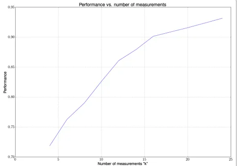
We start by showing the performance of the algorithm vs. the number of measurementskwhere the extracted fea-tures are from. The size of the feature vector changes byk
and the table shown in Table 1 fork=10. The data we use are simulated data from a controlled random walk. The controlled random walk consists of a three-state transition matrix which has a deceleration state, steady state, and acceleration state. The parameters for maximum and min-imum speed are incorporated which changes the proba-bility in the transition matrix if the speed is not within the boundary of the permitted speed range. The data for
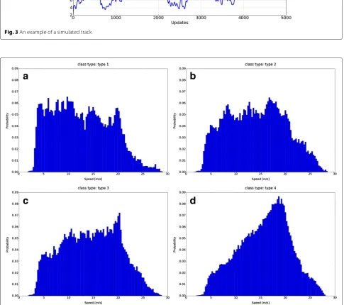
Fig. 3An example of a simulated track
different targets are generated such that they have nearly the same support in speed and the main difference is the acceleration support. The random walk creates positions
pxm and pym which are extrapolated from some smooth speedsvˆxmandˆvymdescribed later.
pxm=pxm−1+tvˆxm+mx (23)
pym=pym−1+tvˆ y
m+my, (24)
wheretis the time between the updates formandm−1 andmx andymare position uncertainties drawn from a distribution.
x m
y m
∼N(0,e), (25)
whereeis the position covariance andN denotes the normal distribution. The smooth speeds are speeds vxm
andvymwhich are convolved with a 25-tap moving average filterh. This is done to avoid quick changes in the speed.
ˆ
vxm=h∗vxm (26)
ˆ
vym=h∗vym. (27)
The speeds (27) are extrapolated from accelerations
axj(m) andayj(m), where j denotes depending upon the statejdescribed in (32). The speeds are given as
vxm vym
= vxm−1+toxj(m)
vym−1+toyj(m),
(28)
whereoxj(m)andoyj(m)are accelerations which are drawn from two normal distributions given by
oxj(m)∼Nμx,j,σx2,j
(29)
oyj(m)∼N
μy,j,σyy,j
(30)
The parameters for the normal distribution μx,j, μy,j,
σ2
x,j, andσy2,j are given from the functionφj(v(m−1),). This is done because we want to control the maximum and minimum allowed speed. We define this function as
φj(v(m−1),)= ⎧ ⎨ ⎩
ψj(1) ifvm−1> ζmax,
ψj(2) ifζmin≤vm−1≤ζmax
ψj(3) else,
,
(31)
where ψj(1), ψj(2), andψj(3) are the set of parameters
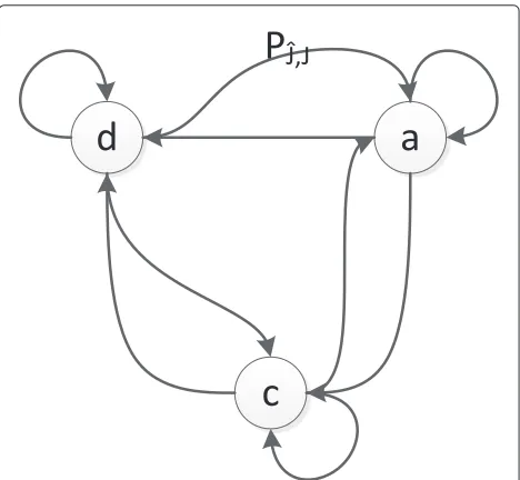
{μy,j,μx,j,σy2,j,σx2,j}used in (30) and = {ζmin,ζmax}. The state machine consists of three states: deceleration (d), constant(c), and acceleration(a) states, see Fig. 2. Fur-ther, the state machine is also controlled by the speed. We define the state transition probabilities as
Pˆj,j(v(m−1),)= ⎧ ⎪ ⎨ ⎪ ⎩
ˆj,j(1) ifvm−1> ζmax,
ˆj,j(2) ifζmin≤vm−1≤ζmax
ˆj,j(3) else,
,
(32)
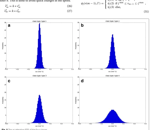
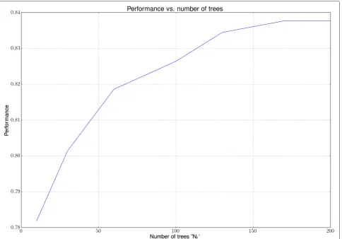
whereˆjis the previous state andˆj,jis the transition prob-ability. An example of a track can be seen in Fig. 3. The speed PDFs can be seen in Fig. 4, and the accelerations PDF can be seen in Fig. 5. The performance of the clas-sifier vs. the number of measurementsk can be seen in Fig. 6. Further, we show the performance of the classifier vs. the number of treesNtused in the random forest, see Fig. 7. The confusion matrix of the classification results for the four classes can be seen in Table 2, where we have usedk=10 andNt=100.
4 Real-world results
The data used for this work consist of Automatic Identifi-cation System (AIS), which is a broadcast system used for large ships; Automatic Dependent Surveillance-Broadcast (ADS-B), which is a broadcast system used for commercial aircrafts; GPS logs; and real-world radar data. The classes for this work are typical classes for coastal surveillance, e.g., large ships, birds, and small boats.
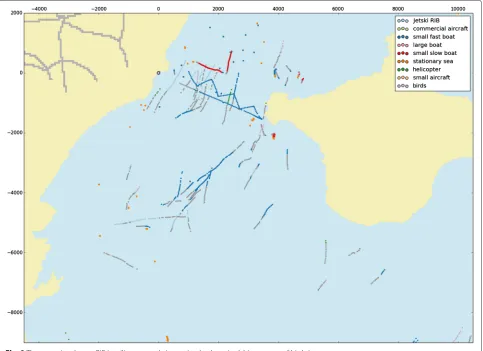
We show a confusion matrix for real-world data in Table 3. As a confusion matrix does not take into account how the probability develops over time, we also show some real-world scenarios. For these scenarios, extra classes are used. The scenarios are images showing all tracks within a specific time period. The scenarios have both known and unknown targets. It is therefore not pos-sible to make a confusion matrix of the scenario; however, it is possible to have a good estimate of the performance of the classifier in real-world situations. The scenarios are recorded with different radars and antennas; further, the sampling rate can be different for the different scenarios. We show two scenarios from coastal surveillance applica-tions. The first coastal surveillance scenario is recorded in
Fig. 7The performance of the classifier for the synthetic generated data vs. the number of trees used in the random forest
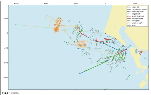
Denmark where a rigid inflatable boat (RIB) is sailing from west to east and zigzagging back. Towards the north of the RIB, there are two unknown vessels; further, there are some sea buoys present both to the north of the RIB and also to the far south. The rest of the tracks are believed to be birds. See the scenario in Fig. 8. The second scenario is also from Denmark and shows two wind turbine farms. A commercial plane is flying in from the west to the east, and a small personal aircraft is circling over the first wind farm to the north, then the second wind farm, and finally leaving towards the east. Three vessels are present, one to
Table 2The confusion matrix of the simulated data
Predicted
Actual Type 1 Type 2 Type 3 Type 4
Type 1 95.2 4.8 0.0 0.0
Type 2 16.7 72.1 11.2 0.0
Type 3 1.0 35.6 63.3 0.0
Type 4 0.0 0.0 0.0 99.9
Overall performance 82.6
the east of the wind farm in the north (above the other wind farm) and the second vessel is sailing through the wind farm in the south. The last vessel is sailing from west to east under the south wind farm. The rest of the tracks are believed to be birds, see Fig. 9. As the majority of pre-viously published results are based on a joint tracking and classification approach, mostly on simulated data, it is not directly possible to compare the obtained classification accuracy.
In the next section, we will discuss the results of the classifier.
5 Discussion
Table 3The confusion matrix for real-world data
Predicted
Actual Birds RIBs Stationary sea Large ships Helicopters Commercial aircrafts targets
Birds 67.9 9.2 0.0 21.0 1.9 0.0
RIBs 6.4 62.4 0.0 31.2 0.0 0.0
Stationary sea targets 0.5 0.0 99.5 0.0 0.0 0.0
Large ships 21.4 5.1 0.3 61.5 11.6 0.0
Helicopters 12.2 0.0 0.0 0.0 87.8 0.0
Commercial aircrafts 0.8 0.0 0.0 0.0 0.0 99.2
Overall performance 79.7
increasing the number of measurements is that it takes longer time from a track is seen until the first probability of the target is shown. For our results, the sampling rate varies between 0.333 and 1 Hz. For 10 measurements, this gives a maximum waiting time of 30 s, which we believe for the application in hand is acceptable. In Fig. 7, the per-formance can be seen when varying the number of trees used in the random forest. The plot is made withk =10.
It can be seen that the performance does not get better after around 170 trees. The increase in the number of trees takes longer time to train the random forest and is more computationally expansive and memory requiring when using the classifier for testing, i.e., the purpose of the clas-sifier is to run in real time. The performance ofk = 10 andnt = 100 can be seen in Table 2. It is clear that type 2 and type 3 have the most confusion between them. This
Fig. 9Horns Rev
is also natural if we look at the speed PDFs and the accel-eration PDFs in Figs. 4 and 5, respectively, as these are very similar. In general, the diagonal numbers in the con-fusion matrix are at the left side. This is due to the fact the large allowed acceleration still contains smaller accel-eration which therefore will be classified as a lower class type.
For the real-world scenarios, we usek = 10 andnt = 170. As it can be seen, the confusion matrix in Table 3 shows relative good performance. Nearly all of the sta-tionary sea targets and commercial aircrafts are classified correctly. The helicopters are confused with birds. This can be because the helicopters can move as slow as birds. There is some confusion between large ships, birds, and RIBs. All of these classes have kinematics which are close to each other.
In Fig. 8, one of the real coastal surveillance scenarios is shown. The scenario shows a RIB sailing out from a marina and zigzagging back again. The RIB is classified as a small fast boat. The reason that it is not classified as a Jet Ski/RIB is that it sails more like a fast boat whereas a Jet Ski/RIB often makes turns, accelerates, and deceler-ates. The two slow-moving vessels to the north of the RIB are classified correctly. Some of the sea buoys are classified correctly as stationary targets. Only a few birds are clas-sified correctly. In Fig. 9, two wind farms can be seen and nearly all of the wind turbines are classified as stationary,
while a few are misclassified as small slow-moving boats. The commercial aircraft is between a commercial aircraft and small aircraft; however, the target is primarily classi-fied as a commercial aircraft. The small aircraft circling the two wind farms is classified correctly even though the aircraft is flying below stall speed. This can be due to the strong winds, and therefore, the real airspeed is much larger. The one sea vessel that is sailing between the wind turbines is misclassified as a bird, while the other sea ves-sels are classified as small slow boats, small fast boats, and helicopters. Unfortunately, nearly all the birds are misclas-sified either as unknown or as a helicopter. We believe this is because the training data do not contain any birds at that distance and speed (because of the wind). Further, the radar used to record this scenario is different from the radars used for the training data.
6 Conclusions
Acknowledgements
This work was partially supported by the Engineering and Physical Sciences Research Council (EPSRC) Grant number EP/K014307/1 and the MOD University Defence Research Collaboration in Signal Processing.
Competing interests
The authors declare that they have no competing interests.
Author details
1Terma A/S, Hovmarken 4, Lystrup, Denmark.2Department of Electronic
Systems, Aalborg University, Fredrik Bajers Vej 7b, Aalborg, Denmark.
3Technology & Innovation Centre, University of Strathclyde, 99 George St,
Glasgow, Great Britain.
Received: 31 March 2016 Accepted: 6 July 2016
References
1. LW Jochumsen, M Pedersen, K Hansen, SH Jensen, J Østergaard, inRadar Conference (Radar), 2014 International. Recursive Bayesian classification of surveillance radar tracks based on kinematic with temporal dynamics and static features (IEEE, Lille, France, 2014), pp. 1–6
2. LW Jochumsen, E Nielsen, J Østergaard, SH Jensen, M Pedersen, inRadar Conference (RadarCon), 2015 IEEE. Using position uncertainty in recursive automatic target classification of radar tracks (IEEE, Washington DC, USA, 2015), pp. 0168–0173
3. DH Nguyen, JH Kay, BJ Orchard, RH Whiting, Classification and tracking of moving ground vehicles. Lincoln Lab. J.13(2), 275–308 (2002)
4. S Challa, GW Pulford, Joint target tracking and classification using radar and ESM sensors. IEEE Trans. Aerosp. Electron. Syst.37(3), 1039–1055 (2001)
5. D Angelova, L Mihaylova, Joint target tracking and classification with particle filtering and mixture Kalman filtering using kinematic radar information. Digital Signal Process.16(2), 180–204 (2006)
6. Z Sun, XJ Ban, Vehicle classification using GPS data. Transp. Res. Part C Emerg. Technol.37, 102–117 (2013)
7. M Garg, U Singh, inNational Conference on Research Trends in Computer Science and Technology (NCRTCST), IJCCT_Vol3Iss1/IJCCT_Paper_3. C & R tree based air target classification using kinematics (IJECCE, Hyderabad, India, 2012)
8. L Breiman, Random forests. Mach. Learn.45(1), 5–32 (2001)
9. S Theodoridis, K Koutroumbas,Pattern Recognition, Fourth Edition, 4th edn. (Academic Press, 2008)
10. E Brookner,Tracking and Kalman Filtering Made Easy. (Wiley-Interscience, 1998)
11. J Friedman, T Hastie, R Tibshirani,The Elements of Statistical Learning, vol. 1. (Springer, 2001)
12. CM Bishop,Pattern Recognition and Machine Learning, vol. 1. (Springer, New York, 2006)
13. G James, D Witten, T Hastie,An Introduction to Statistical Learning: with Applications in R. (Taylor & Francis, 2014)
14. L Chen, S Wang, inProceedings of the 21st ACM International Conference on Information and Knowledge Management. Automated feature weighting in naive bayes for high-dimensional data classification, (ACM, 2012), pp. 1243–1252
15. JA Lawton, RJ Jesionowski, P Zarchan, Comparison of four filtering options for a radar tracking problem. J. Guid. Control. Dyn.21(4), 618–623 (1998) 16. N Mohajerin, J Histon, R Dizaji, SL Waslander, inRadar Conference, 2014
IEEE. Feature extraction and radar track classification for detecting UAVs in civillian airspace, (2014), pp. 0674–9
17. SWBD. http://dds.cr.usgs.gov/srtm/version2_1/SWBD/. Accessed 4 Dec 2014
Submit your manuscript to a
journal and benefi t from:
7Convenient online submission
7Rigorous peer review
7Immediate publication on acceptance
7Open access: articles freely available online
7High visibility within the fi eld
7Retaining the copyright to your article