R E S E A R C H
Open Access
Random filtering structure-based compressive
sensing radar
Jindong Zhang
*, YangYang Ban, Daiyin Zhu and Gong Zhang
Abstract
Recently with an emerging theory of ‘compressive sensing’ (CS), a radically new concept of compressive sensing radar (CSR) has been proposed in which the time-frequency plane is discretized into a grid. Random filtering is an
interesting technique for efficiently acquiring signals in CS theory and can be seen as a linear time-invariant filter followed by decimation. In this paper, random filtering structure-based CSR system is investigated. Note that the sparse representation and sensing matrices are required to be as incoherent as possible; the methods for optimizing the transmit waveform and the FIR filter in the sensing matrix separately and simultaneously are presented to decrease the coherence between different target responses. Simulation results show that our optimized results lead to smaller coherence, with higher sparsity and better recovery accuracy observed in the CSR system than the nonoptimized transmit waveform and sensing matrix.
Keywords: Compressive sensing radar; Random filtering; Cross-correlation; Optimization algorithm
1 Introduction
Compared with the whole scene observed by radar sys-tems, the target scene is sparse therein in the majority of cases. Classical radars do not take advantages of this spar-sity and lead to complicated and expensive radar receiver consisting of high-rate analog-to-digital (AD) converters, large memories, and fast computing systems.
Recently with an emerging theory of ‘compressive sens-ing’ (CS) [1-4], a radically new concept of compressive sensing radar (CSR) has been proposed [5]. According to CS theory, CSR can recover the target scene from far fewer samples or measurements than traditional methods. To make this possible, CSR relies on two principles: sparsity, which restricts the number of targets of interest, and inco-herence, which says the dissimilarity between targets of interest. Obvious characteristics of the CSR system can be summarized as follows [5,6]:
• Eliminating the need for the pulse compression matched filter at the receiver
*Correspondence: [email protected]
College of Electronic and Information Engineering, Nanjing University of Aeronautics and Astronautics, Nanjing, Jiangsu 210016, People’s Republic of China
• Reducing the required receiver AD conversion bandwidth so that it need operate only at the low ‘information rate’ rather than at the high Nyquist rate
• Providing the potential to achieve higher resolution between targets than traditional radars whose resolution is limited by the uncertainty principles
Two different tasks of CSR have been investigated by only a few papers. The first radar task is to detect and estimate targets in distinct range, Doppler and angle cells [6,7]. The second is imaging, including range profiling, synthetic aperture radar (SAR) and inverse synthetic aper-ture radar (ISAR) [8-10]. In both cases, CSR can work in the situation of sparse targets/scene. CSR was demon-strated to be capable of successfully working with an AD converter operating at a sampling frequency lower than the Nyquist rate. An exact recovery of target scene can be implemented with four times undersampling for CSR SAR imaging [5]. CSR was considered to transmit a sufficiently incoherent pulse and reconstruct the sparse target scene by the greedy algorithm. Better resolution in the time-frequency plane over traditional radar can be provided [6]. In [8-10], CS technique was applied to range profiling, azimuth domain focusing, and(ω,k)domain focusing in SAR imaging.
CSR waveform design was also investigated by Chen [11] and Subotic [7]. To effectively reconstruct the target scene, it is required that the correlations between tar-get responses must be small. A input multiple-output (MIMO) radar waveform design method has been proposed based on simulated annealing (SA) algorithm [11]. For a distributed radar system, waveform and posi-tion impacts have been examined by consideraposi-tions of sparsity of the target scene and the restricted isometry property (RIP) [7], [12].
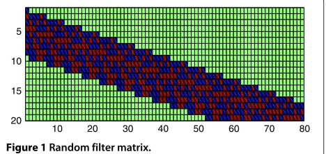
In [5], Baraniuk has suggested an interesting choice for the sensing matrix of CSR system. He pointed out that in majority of cases we can use a causal, quasi-Toeplitz matrix where each row is a right shift of the row imme-diately above it. The sensing matrix based on random filtering is plotted in Figure 1. The measurement process in CSR can be seen as a linear time-invariant filter fol-lowed by decimation. When we choose a pseudo-noise (PN) sequence as the initial row, this approach can be named as random filtering. Obvious benefits of random filtering structure-based CSR can be summarized as [13]
• The sensing matrix is stored and applied efficiently.
• Fast fourier transformation (FFT) can be used to replace convolution for long filters.
• It is easily implementable in software or hardware.
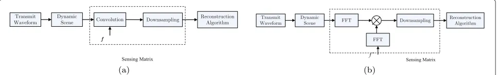
The constitutions of the two kinds of random filtering structure-based compressive sensing radar is illustrated in Figure 2. As we can see, the random filter can be imple-mented both in time and frequency domain. In Figure 2, we also note that two Toeplitz matrices have been used and concatenated. The first appears due to the convolu-tion of the transmitted waveform with the sparse target scene, spreading the energy of each target in the scene. The second is caused by the convolution of a random filter with the received signal. Actually, the input for the second Toeplitz matrix is no longer sparse in the canonical basis because of the concatenation of the two matrices.
CS theory suggests that the sensing matrixand sparse representation matrix be as incoherent (orthogonal) as
10 20 30 40 50 60 70 80
5
10
15
20
Figure 1Random filter matrix.
possible. A measure of coherence betweenandcan
be expressed as
ρ(,)=max
i=j |i,j| (1)
where,denotes the inner product,iis theith row of, andjis thejth columns of.ρ(,)plays an important role in the successful recovery of basis pursuit (BP) and orthogonal matching pursuit (OMP) algorithms [14]. Low
coherence betweenandmeans smallρ(,).
We note that a key notion of the RIP in CS theory also requires the orthogonality betweenand[15]. The RIP can be expressed as [16]
∀|T| ≤S:(1−δS)θT22≤ DTθT22≤(1+δS)θT22 (2)
where ∀|T| ≤ S mean for any sparsityT, which is less thanS,| · |is the cardinality operator, · 2represents the l2 norm being equivalent to the square root of the sum
of squares of all the elements,D = is the
equiva-lent dictionary,DT is a subset extracted fromD,θT are
the coefficients corresponding to theTselected columns, and 0 < δS < 1 is the S-restricted isometry constant
(RIC). If the RIP holds, any subset of columns of Dare
nearly orthogonal and the incoherence between and
is ensured. However, the RIP is difficult for us to ver-ify [17]. Therefore, some matrices have been proved to be incoherent enough with any fixed sparsifying basis
with overwhelming probability, such as Gaussians or±1 random matrices [16].
Elad has proposed an alternative framework towards the incoherence required by CS [18]. This alternative, which has been shown to be computationally more efficient and produce significantly better results, can be described as [19]
theith column ofD. The mutual coherence is known to be a sub-optimal metric to quantify CS matrices as com-pared to RIC. Notably,μ≥1/√Mfor aM×NGaussian matrix. Thus, using the mutual coherence metric, we have a sub-optimal quadratic scaling ofMwith the sparsityS. In comparison, a linear scaling ofMwithSis achieved with the RIC.
IfDis designed such thatμ(D)is as small as possible,
the orthogonality between and can be guaranteed
Figure 2The constitution of random filtering structure-based compressive sensing radar.Random filter can be implemented in time and frequency domain:(a)time domain random filter with convolution and(b)frequency domain random filter with FFT and IFFT.
In this paper, we are concerned with incoherence between the sensing and sparse representation matrices in random filtering structure-based CSR. With the thought that the sensing matrix and transmit waveform in CSR can be changed in mind, we will investigate the problem of how to design the sensing matrix and transmit waveform to guarantee incoherence in the CSR system.
A similar thought has appeared in image processing and can be traced back to Elad’s work [18]. Elad first attempted to decrease the average mutual coherence by optimizing the sensing matrix. His work showed that designing a sensing matrix is a better choice than a ran-dom matrix, and it indeed leads to better CS perfor-mance. Abolghasemi proposed a gradient descent method to optimize the sensing matrix [20]. Duarte-Carvajalino extended Elad’s work and proposed to optimize the sparse representation and sensing matrices simultaneously [15]. Due to more freedom degrees introduced in CS, this new CS framework can offer better performance than only optimizing the sensing matrix. Overall, the results of these methods show enhancement in terms of both reconstruc-tion accuracy and the maximum allowable sparsity CS can recover.
The remainder of this paper is organized as follows. First, we study the theory of random filtering structure-based compressive sensing radar in Section 2. Then, we introduce our proposed algorithms to design the transmit waveform and sensing matrix in Section 3. In Section 4, we present detailed experimental results demonstrating the superiority of our framework. Finally, concluding remarks and directions for future research are presented.
2 Review of compressive sensing radar based on
random filtering
2.1 Sparse representation dictionary
Consider a target scene in time-frequency plane is
dis-cretized into an L × M grid, and we define time and
frequency shift matrices as
TlL×N =
whereLandMdenote the numbers of range and Doppler
bin CSR measures, N is the length of transmit
wave-form vector, ωM = e
√
−12π/M is theMth root of unity.
The(l,m)th basis element in time-frequency plane can be defined as
pl,m=Fm·Tl (6)
where l = 1, 2,. . .,L, m = 1, 2,. . .,M. Assuming the transmit signalxof lengthN, the receiver will receive a signalhl,m =pl,m·xof lengthLto observeLrange bins.
Note that there are necessarily LMgrid points in time-frequency plane; we concatenate these received signals and obtain the received signal basis dictionary
=(h1,1|h1,2| · · · |hL,M)
=Hx (7)
where
H=(p1,1|p1,2| · · · |pL,M)
is the product we define as
(A|B)s=(As|Bs)
AandBare matrices of the same sizem×nandsis a vector of sizen×1. The sparse representation dictionary
contains all the possible signal reflected from the target in any grid of time-frequency plane.
2.2 Random filtering measurement
In CS, the sensing matrix measures and encodesP < L
linear projections of the signal. By random filtering mea-surement, this process can be seen as the convolution of the received signal and the FIR filterfof lengthB, which approximates the analog filtering in the digital domain. To takePmeasurements of the signal, downsampling of the FIR filter output is then carried out. This process can be
represented by a matrix , where is aP ×Lmatrix.
This matrix is banded and quasi-Toeplitz: each row hasB
By the fixed filter f which is defined on the region floor function. Thepth row ofcan be expressed as
(T)p=Mpf
Mpis aL×Bmatrix with the following expression
Mp=
The received signal of the target scene can be expressed as
r=
cient vector of the scene andnis the additive Gaussian white noise vector of length L. The measured signal is written as
y=r=θ +n (10)
Then, the target scene can be recovered by reconstruc-tion methods including using algorithms such as orthogo-nal matching pursuit [21,22] and basis pursuit [23,24]. The latter program is solving the following convex problem:
minθ1 s.t.y−θ22≤ (11)
where·1denotes thel1norm of a vector or matrix which is equal to the sum of absolute value of all the elements and
>0 takes into account the possibility of noise in the lin-ear measurements and of nonexact sparsity. Regularized orthogonal matching pursuit (ROMP) has been proposed to take advantage of OMP and BP algorithms [25].
3 The FIR filter and transmit waveform design for compressive sensing radar
Equation 3 defines the maximum absolute value of nor-malized inner product between all columns in the equiva-lent dictionaryD. Suppose the sparsity of the target scene θ0satisfies the following inequality
θ0< 1 nonzeros in a vector or matrix.θis necessarily the sparsest solution (minθ0) such thaty=Dθ.
A fast greedy algorithm such as OMP is guaranteed to succeed in finding the correct solution in the presence
of noise n. The root mean square error (RMSE) of the
solutionθobeys [14]
θ−θ2≤ √ (δ+)
1−μ(D)(2θ0−1) (13)
where = n2andδ ≥ = y−Dθ2. The mutual
coherenceμ(D)that affects both the recoverable sparsity of target scene and the recovery accuracy is demonstrated in (12) and (13).
We note that in the equivalent dictionaryD, the FIR fil-terfin the sensing matrixand the transmit waveform xare variables in the CSR system. Therefore, the FIR fil-terfand transmit waveformxdesign problem in the CSR system can be described as
argmin
where(·)Hdenotes the conjugate transposition. Here, we replace the transposition(·)T in Equation 3 by the con-jugate transposition (·)H to process the columns of the complex equivalent dictionaryDin the CSR system.
3.1 The transmit waveform optimization
With the fixed FIR filterf, the transmit waveformx opti-mization problem can be given by
argmin
μi,j is a variable correlated with the cross-correlations between di and dj and the auto-correlations of di, dj.
We use the square ofμi,j and transform this fraction in
(15) into a weighted summation. This expression can be obtained by
γi,j= dHi dj22−λdi22dj22 =xHPi,jx−λ·xHQix·xHQjx
(16)
whereλis the weighted coefficient,
This transformation is valid by taking the log in (15) (due to the monotonicity of the log function). The optimization problem in (15) can be transformed to
argmin
This minimax problem is difficult for us to solve, and
we replace by minimum summation of γi,j and can be
described as
This transformation is also valid because it is noted that for any vectorx ∈ RN, we have 1/√Nx2 ≤ x∞ ≤ x2. Thus, the optimization problem is simplified to the minimization problem defined in (18), in which the transmit waveformxhas constant energy constraint
xHx=E0
When the transmit vector x is equal to the
eigenvec-tor of corresponding to the smallest eigenvalue, the
minimization ofxHxin (18) is achieved subject to the
energy constraint of xHx = 1. However, the matrix
which depends onxlead to indirect solution. Therefore, an iterative procedure must be applied. The specific steps involved in this iterative procedure are described below:
• Step A1: Set thexwith random generated values or use some existing sequence (i.e., Frank sequence or Golomb sequence),k=0.
• Step A2: Compute the matrixk+1in terms ofxk.
• Step A3: Find the smallest eigenvalue and the corresponding normalized eigenvectorvk+1of the matrixk+1.
• Step A4: Repeat the above steps until the convergence criteria is satisfied, e.g.,xk−xk+12< 1, where xk+1=vk+1is the waveform obtained at thek th iteration and1is a predefined threshold.
3.2 The FIR filter optimization
We define the complex Gram matrixG = DHDwhose
entry at theith row andjth column isgi,j. Unlike the Gram
matrix definition in [18], we do not compute G using
the matrix D after normalizing each of its columns. In practice, the small absolute off-diagonal elements inGis
desired. In the ideal case, minimum possible coherence occurs whengi,j=0,i=j, and we have
whereGis aLM×LMdiagonal matrix with self-coherence of each columns. We might be able to design the
sens-ing matrix making the Gram matrixG close toGas
possible. This process can be written as follows:
argmin
G−G2F (20)
where · F is the Frobenius norm for a matrix. By (10)
and (11), the Gram matrix can be rewritten as
G=DHD=()H
=HH (21)
According to (20), the sensing matrix optimization
problem with the fixed sparse representation matrix
can be described as
argmin
HH−G2
F (22)
With the successful case in [26], simpler criteria can be given to replace (22) and written as
argmin
−Ug2F (23)
whereUis aP×Nsemiunitary matrix (i.e.,UHU=I),g= Diag(√g11,√g22,. . .,√gNN), Diag(·)denotes the diagonal
matrix with diagonal elements as indicated.
Considering the sensing matrixalso has energy con-straint, the above criteria can be rewritten as
argmin
andUare both unknown variables in (24). Our strategy to solve this minimization problem is calculating one vari-able while the other is fixed and iterating this process until convergence appears.
First, we consider the minimization problem with the known sensing matrixin (24) has the following solution [27]
U=UH2U1 (25)
whereU1andU2can be obtained by the following singular value decomposition (SVD) expression
here U1 is a P × P unitary matrix, U2 is an P × LM
semiunitary matrix, andis aP×Pdiagonal matrix.
Then, we try to find f which determines the sensing
matrixwith givenU. We decompose the sensing matrix by rows and have
fT
MT1MT2 · · ·MTP
=vec(Ug)T (27)
After transforming the above expression, we obtain
Af=b (28)
where
A=T
MT1 MT2 · · · MTP T
(29)
b=vec(Ug) (30)
The FIR filterfcan be obtained by the least square (LS) estimator
f=(AAH)−1Ab (31)
The FIR filter foptimization method can be
summa-rized as follows:
• Step B1: Generate the FIR filterfwith random complex values, then compute the initial sensing matrix, setk=0.
• Step B2: Compute the SVD ofkg−1k and the unitary matrixU.
• Step B3: Compute the FIR filterfk+1that minimizes (24) by (31); under the constraintfk+122=c,
fk+1= cfk+1
fk+122
.
• Step B4: Repeat the above steps until the convergence criteria is satisfied, e.g.,fk−fk+12< 2, wherefk+1 is the FIR filter obtained at thek+1th iteration and 2is a predefined threshold.
BecausePLM, the SVD of theP×LMmatrixg−1
in Step B2 requires a large computation amount for large values ofLandM.
3.3 Joint optimization
With the above discussion, now we turn to the transmit waveform xand FIR filterf joint optimization problem. The method will be considered to combine the introduced iterative approaches for optimizing the transmit wave-form and FIR filter. Considering these two variables can-not be optimized simultaneously in an iteration, we split each iteration into two parts, which optimize one variable while the other is fixed. With the transmit waveform and
0 0.1 0.2 0.3 0.4 0.5 0.6 0.7 0.8 0.9 1 0
2 4 6 8 10 12
Normalized cross correlation
Statistic value(%)
0 0.1 0.2 0.3 0.4 0.5 0.6 0.7 0.8 0.9 1 0
2 4 6 8 10 12
Normalized cross correlation
Statistic value(%)
0 0.1 0.2 0.3 0.4 0.5 0.6 0.7 0.8 0.9 1 0
2 4 6 8 10 12
Normalized cross correlation
Statistic value(%)
0 0.1 0.2 0.3 0.4 0.5 0.6 0.7 0.8 0.9 1 0
2 4 6 8 10 12
Normalized cross correlation
Statistic value(%)
(a) (b)
(c) (d)
0 0.1 0.2 0.3 0.4 0.5 0.6 0.7 0.8 0.9 1 0
2 4 6 8 10 12
Normalized cross correlation
Statistic value(%)
0 0.1 0.2 0.3 0.4 0.5 0.6 0.7 0.8 0.9 1 0
2 4 6 8 10 12
Normalized cross correlation
Statistic value(%)
(a) (b)
Figure 4Histogram of the cross-correlations between different target responses.(a)Alltop sequence + optimized sensing matrix and (b)optimized transmit waveform + optimized sensing matrix.
FIR filter optimization approaches in Sections 3.1 and 3.2, the joint optimization method can be summarized as
• Step C1:k=0, generate the transmit waveformxk with random complex values and constant energy, and set the FIR filterfkwith random complex values; compute the corresponding sensing matrixk, the sparse representation matrixk, the equivalent dictionaryDk, and the Gram matrix
Gk=DHkDk.
• Step C2: Assume the deterministic sensing matrix =k, optimize the transmit waveform using Step A2 to Step A4, and obtainx.
• Step C3: With the deterministic waveformx=x, optimize the FIR filter using Step B2 to Step B4 and obtainf.
• Step C4:k=k+1,
xk+1=x
fk+1=f.
• Step C5: Compute the Gram matrix
Gk+1=DHk+1Dk+1.
Repeat the above steps until the convergence criteria is satisfied, e.g.,Gk−Gk+12< 3, where3is a predefined threshold.
The proposed three algorithms in this section is stopped whenever the innovations is less than a certain value (1,2, and3, respectively). The order of the magnitude of these values will be given in the simulation section. Similarly, the number of iterations will also be tested.
4 Simulation
In this section, we will complete computer simulations with three aspects. First, simulation examples will be given to demonstrate the effectiveness of our proposed methods
for decreasing the coherence between the sparsifying rep-resentation and sensing matrices. Second, in CS theory, RIP is an important rule. Simulation results will show that our designed result can ensure this rule finely. Third, the target scene recovery experiment will be given to show the improved recovery accuracy by our methods.
4.1 Transmit waveform and sensing matrix optimization results
The CSR system transmits a waveform of lengthN = 19
and measures a target scene withL=80 range andM=1 Doppler bin. The sensing matrix compresses the received signal with the FIR filterfof lengthB=40 and obtains the measured data of lengthP=40. We optimize the transmit waveformxand FIR filterfof the CSR system separately and simultaneously, and results are compared for these different approaches. The parameters1,2, and3are set to be 10−8, 10−5, and 10−5, respectively. These algorithm will stop after hundreds of iterations in our simulations. The recovery algorithm used here is OMP.
In [6], Herman has proved that the Alltop sequence has nearly ideal incoherence properties for the dictionary. This sequence is defined as
sn=
1 √
Ne √
−12π
Nn3
where n ≥ 5 is a prime. Considering the
impor-tant property of the Alltop sequence, we use it as a
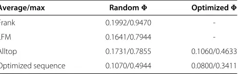
Table 1 Average and maximum values of the cross-correlations
Average/max Random Optimized
Frank 0.1992/0.9470
-LFM 0.1641/0.7944
-Alltop 0.1731/0.7855 0.1060/0.4633
Figure 5The smallest and largest eigenvalues (λmin,λmax).(a)Alltop sequence + random sensing matrix and(b)optimized transmit waveform + optimized sensing matrix.
standard sequence for comparing with our optimization result. In the process of the sensing matrix optimiza-tion, we also use this sequence as the fixed transmit waveform.
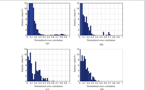
Figure 3 shows the histogram of the cross-correlations between different target responses with random sens-ing matrix. The optimized waveform is compared with the Frank, LFM, and Alltop sequences. As a stan-dard sequence, the maximum and average values of the histogram of the Alltop sequence obviously outper-form Frank and LFM sequences. However, our proposed method can provide a sequence with better performance than the Alltop sequence. The average and maximum
cross-correlations are decreased about 0.07 and 0.27, respectively.
In Figure 4a, the result for the optimized sensing matrix is given. The Alltop sequence is used as the fixed trans-mit waveform. As we can see, the cross-correlations of the optimized sensing matrix are obviously smaller than that of the random matrix. The average and maximum cross-correlations are lowered about 0.17 and 0.32, respectively. The result for the optimized transmit waveform and sensing matrix are also shown in Figure 4b. Compared with that of the Alltop sequence with random sensing matrix, the average and maximum cross-correlations are decreased about 0.09 and 0.44, respectively.
5 10
15 20 25
5 10 15 20 250 0.2 0.4 0.6 0.8 1
(a)
5 10
15 20 25
5 10 15 20 250 0.2 0.4 0.6 0.8 1
The detailed information of the cross-correlations is summarized in Table 1. From the above results, we may conclude that the sensing matrix optimization offers greater performance improvement than the optimized transmit waveform because it can provide more optimiza-tion variables.
whereλminandλmaxare the smallest and largest eigenval-ues ofDHTDT. TheS-restricted isometry constant can be
obtained by
1−δS≤λmin 1+δS≥λmax
(34)
With the constraint 0 < δS < 1 [15], the eigenvalues λminandλmaxshould satisfy
0< λmin≤λmax<2 (35)
Thus, to verify if the equivalent dictionary DT
satis-fies the RIP, we should compute the eigenvaluesλminand λmax of all the possible subset matrix DT. This
opera-tion needs great amount of computaopera-tion. We use 1,000 times Monte Carlo simulations instead. The smallest and
10 12 14 16 18 20 22 24 26 28
largest eigenvalues (λmin,λmax) are plotted in Figure 5. As we can see, (35) holds with the sparsity K ≤ 3 for All-top sequence and random filtering measurement matrix. However, with optimized transmit waveform and FIR fil-ter, (35) can be satisfied until the sparsity is increased to 8. We note that this simulation does not verify the RIP but instead provides to proxy to it.
4.3 Target scene recovery
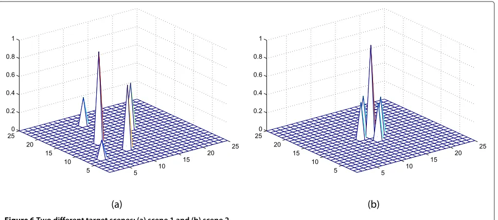
To verify the effectiveness of the transmit waveform and sensing matrix optimization in random filtering structure-based CSR system, we assume that a sparse target scene hasL=25 range andM=25 Doppler bins. The CSR sys-tem transmits a waveform of lengthN=31 and measures the received signal with a sensing matrix ofP×L, where
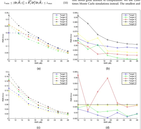
P=25. There are two target scenes in Figure 6. The scene is recovered by the Alltop sequence and random sens-ing matrix or optimized waveform and senssens-ing matrix, and this process is carried out by 1,00 times. Figure 7 shows the root mean squared (RMS) errors of the recov-ery results of the two target scenes versus SNR. As we can see, recovery errors with optimized waveform and sensing matrix are much smaller than the result with All-top sequence and random sensing matrix. With increased SNR, the recovery error is obviously decreased.
5 Conclusions
A new notion of random filtering structure-based com-pressive sensing radar was proposed in this paper. To decrease the coherence between the sparse represen-tation and sensing matrices, a compurepresen-tational frame-work for optimizing the transmit waveform and sensing matrix separately and simultaneously was introduced. We showed that optimized transmit waveform and sensing matrices lead to smaller mutual coherence between differ-ent target responses. We also use Monte Carlo simulations to verify whether our optimized results satisfy RIP. Sim-ulation results demonstrate that our optimized results can obey RIP with much higher sparsity than nonopti-mized waveform and sensing matrix. As we can see, the reconstruction accuracy was significantly improved by the optimized transmit waveform and sensing matrices for a given target scene.
Competing interests
The authors declare that they have no competing interests.
Acknowledgements
This work was supported by the Defense Industrial Technology Development Program under grant B2520110008, the National Natural Science Foundation of China under grant 61201367, the Natural Science Foundation of Jiangsu Province under grant BK2012382, the Aeronautical Science Foundation of China under grant 20112052025, and the Fundamental Research Funds for Central Universities (No. NS2013023, NJ20140011).
Received: 14 January 2014 Accepted: 5 June 2014 Published: 17 June 2014
References
1. E Candes, J Romberg, T Tao, Robust uncertainty principles: exact signal reconstruction from highly incomplete frequency information. IEEE Trans. Inf. Theory.52(2), 489–509 (2006)
2. D Donoho, Compressed sensing. IEEE Trans. Inf. Theory.52(4), 1289–1306 (2006)
3. E Candes, J Romberg, Sparsity and incoherence in compressive sampling. Inverse Problems.23(3), 969–985 (2007)
4. E Candes, M Wakin, An introduction to compressive sampling [a sensing/sampling paradigm that goes against the commom knowledge in data acquisition]. IEEE Signal Process. Mag.25(2), 21–30 (2008) 5. R Baraniuk, P Steeghs, Compressive radar imaging, inIEEE Radar
Conference(Boston, 17 Apr 2007), pp. 128–133
6. M Herman, T Strohmer, Compressed sensing radar. IEEE Trans. Signal Process.13(10), 589–592 (2006)
7. N Subotic, B Thelen, K Cooper, W Buller, J Parker, J Browning, H Beyer, Distributed radar waveform design based on compressive sensing considerations, in2008 IEEE Radar Conference(Rome, 2008), pp. 1–6 8. I Stojanovic, WC Karl, M Cetin, Compressed sensing of mono-static and
multi-static SAR., inSPIE Defense and Security Symposium, Algorithms for Synthetic Aperture Radar Imagery(Orlando, 28 Apr 2005),
pp. 7337:733705-1–733705-12
9. I Stojanovic, WC Karl, Imaging of moving targets with multi-static SAR using an overcomplete dictionary. IEEE J. Sel. Topics Sig. Proc.4(1), 164–176 (2010)
10. M Tello, P Lopez-Dekker, J Mallorqui, A novel strategy for radar imaging based on compressive sensing, inIEEE International Geoscience and Remote Sensing Symposium, IGARSS 2008, vol. 2 (Munich, 22 June 2012), pp. II-213-II-216
11. CY Chen, PP Vaidyanathan, Compressed sensing in MIMO radar, in42nd Asilomar Conference on Signals, Systems and Computers(Pacific Grove, 2008), pp. 41–44
12. E Candes, The restricted isometry property and its implications for compressed sensing. Comptes Rendus Methematique.346(9), 589–592 (2008)
13. JA Tropp, M Wakin, M Duarte, D Baron, R Baraniuk, Random filters for compressive sampling and reconstruction, inIEEE Int. Conf. on Acoustics, Speech and Signal Processing(Toulouse, 2006)
14. D Donoho, M Elad, VN Temlyakov, Stable recovery of sparse overcomplete representations in the presence of noise. IEEE Trans. Inf. Theory.52(1), 6–18 (2006)
15. JM Duarte-Carvajalino, G Sapiro, Learning to sense sparse signals: simultaneous sensing matrix and sparsifying dictionary optimization. IEEE Trans. on Image Process.18(7), 1395–1408 (2009)
16. EJ Candès, The restricted isometry property and its implications for compressed sensing. Comptès Rendus Mathématique.346(9–10), 589–592 (2008)
17. C Dossal, G Peyré, J Fadili, A numerical exploration of compressed sampling recovery. Linear Algebra Appl.432(7), 1663–1679 (2010). http://hal. archives-ouvertes.fr/docs/00/43/66/94/PDF/DossalPeyreFadili-LAA.pdf 18. M Elad, Optimized projections for compressed sensing. IEEE Trans. Signal
Process.55(12), 5695–5702 (2007)
19. H Rauhut, Compressive sensing and structured random matrices, in Theoretical Foundations and Numerical Methods for Sparse Recovery, MR2731597, vol. 9 (de Gruyter, Berlin, 2010), pp. 1–92
20. V Abolghasemi, S Ferdowsi, B Makkiabadi, S Sanei, On optimization of the measurement matrix for compressive sensign, in18th European Signal Procesing Conference(Aalborg, 2010), pp. 427–431
21. JA Tropp, AC Gilbert, Signal recovery from partial information by orthogonal matching pursuit. IEEE Trans. Inf. Theory.53(12), 4655–4666 (2008)
22. JA Tropp, Greed is good: algorithmic results for sparse approximation. IEEE Trans. Inf. Theory.50(10), 2231–2242 (2004)
23. SS Chen, D Donoho, MA Saunders, Atomic decomposition by basis pursuit. SIAM Rev.52(2), 489–509 (2001)
24. E Candes, J Romeberg, T Tao, Robust uncertainty principles: exact signal reconstruction from highly incomplete frequency information. IEEE Trans. Inf. Theory.53(12), 4655–4666 (2008)
26. P Stocia, H He, J Li, New algorithms for designing unimodular sequences with good correlation properties. IEEE Trans. Signal Process.57(4), 1415–1425 (2009)
27. P Stocia, J Li, X Zhu, Waveform synthesis for diversity-based transmit beampattern design. IEEE Trans. Signal Process.56(6), 2593–2598 (2009)
doi:10.1186/1687-6180-2014-94
Cite this article as:Zhanget al.:Random filtering structure-based compressive sensing radar.EURASIP Journal on Advances in Signal Processing 20142014:94.
Submit your manuscript to a
journal and benefi t from:
7Convenient online submission
7 Rigorous peer review
7Immediate publication on acceptance
7 Open access: articles freely available online
7High visibility within the fi eld
7 Retaining the copyright to your article