R E S E A R C H
Open Access
Robust motion estimation on a low-power
multi-core DSP
Francisco D Igual
*, Guillermo Botella, Carlos Garc´ıa, Manuel Prieto and Francisco Tirado
Abstract
This paper addresses the efficient implementation of a robust gradient-based optical flow model in a low-power platform based on a multi-core digital signal processor (DSP). The aim of this work was to carry out a feasibility study on the use of these devices in autonomous systems such as robot navigation, biomedical assistance, or tracking, with not only power restrictions but also real-time requirements. We consider the C6678 DSP from Texas Instruments (Dallas, TX, USA) as the target platform of our implementation. The interest of this research is particularly relevant in optical flow scope because this system can be considered as an alternative solution for mid-range video resolutions when a combination of in-processor parallelism with optimizations such as efficient memory-hierarchy exploitation and multi-processor parallelization are applied.
Keywords: Motion estimation, Digital signal processors, Bio-inspired systems
1 Introduction
Motion estimation has been deeply investigated during the last 50 years; however, it is still considered by the scientific community as an emerging field of special inter-est due to the plethora of applications that supports the interpretation of the real world, such as navigation, sports tracking, surveillance, video compression, robotics, vehicular technology, etc. It is also useful in the neuro-science field, where the task of modeling neuromorphic algorithms and systems, which fit well according to the human brain evidences, is an open and common research problem.
Motion estimation determines motion vectors and describes the transformation of an entire two-dimensional (2D) image into another, usually taken from contiguous frames in a video sequence using pixels or specific parts such as shaped patches or rectangular blocks.
Motion relies on three dimensions, but images are a projection of the three-dimensional scene onto a two-dimensional plane, therefore posing a mathemati-cally ill-posed problem [1-3], usually known as ‘aperture problem’. To overcome these drawbacks, external knowl-edge regarding the behavior of objects, such as rigid body constraints or other models that might approximate the
*Correspondence: fi[email protected]
Depto. Arquitectura de Computadores y Autom´atica, Universidad Complutense de Madrid, Madrid 28040, Spain
motion of a real video camera, becomes necessary. These models are based on the motion of rotation, translation, and zoom, in all three dimensions.
Theoptical flowparadigm is not exactly the same con-cept as motion estimation, although they frequently come up associated. Optical flow is the apparent motion of image objects or pixels between frames [3]. Two assump-tions are usually applied to optical flow [4]:
- Brightness constancy: although the 2D position of the image discriminant characteristics, such as brightness, color, etc., may change, they keep their value constant over time. Algorithms for estimating optical flow exploit this assumption in various ways to compute a velocity field that describes the horizontal and vertical motions of every pixel in the image. - Spatial smoothness: it appears from the observation
that pixels in the neighborhood usually belong to the same surface and are inclined to present the same image motion.
Optical flow has many drawbacks that increase the burden of estimating it. For instance, the optical flow is ambiguous in homogeneous image regions due to the brightness constancy assumption. Additionally, in real scenes, the assumption is violated at the motion boundaries as well as by occlusions, noise, illumina-tion changing, reflecillumina-tions, shadows, etc. Therefore, only
the synthetic-made motion can be recovered with no ambiguity. These two assumptions may lead to errors in the flow estimates.
There are a number of common examples which deliver a non-null value for motion estimation but a zero value for optical flow, e.g., a rotating sphere under constant illumi-nation. Similarly, a static sphere with changing light will deliver optical flow, while the motion field remains null [1], or an old barber pole in motion that shows a real velocity field perpendicular to the estimated optical flow.
Classifying the state of the art in algorithms and tech-niques, we find a common taxonomy used to estimate optical flow. They generally fall into one of the following categories:
- Pattern-matching methods [3] are probably the most intuitive methods. They operate by comparing the positions of image structure between adjacent frames and inferring velocity from the change in location. The aim of block-matching methods is to estimate motion vectors for each macro-block within a specific and fixed search window in the reference frame. These exhaustive or semi-exhaustive search algorithms match all macro-blocks within a search window in the reference frame to estimate the optimal macro-block in order to fit with the minimum block-matching error metric.
- Motion energy methods are probabilistic methods
that use space-time oriented filters tuned to respond optimally to specific image velocities. Banks of such filters are used to respond to a range of visual motion possibilities [1]. Therefore, motion estimation is not unique for every single stimulus. These methods usually work under Fourier space.
- Gradient-based or differential technique family uses derivatives of image intensity in space and time. Combinations and ratios of these derivatives yield explicit measures of velocity [2,5]. The particular implementation of the algorithm used in this paper belongs to this family and is based on Johnston’s work [6,7]. Themulti-channel gradient model (McGM) was developed as part of a research effort aimed at improving our understanding of the human visual system. This model also allows us to make predictions that can be tested through psychophysical experimentation as separate motion illusions that are observed by humans in experiments [8].
One of the main drawbacks of the McGM model is the high hardware requirements needed to achieve real-time processing. On one hand, McGM presents an uptrend in temporal data storage which is translated into non-negligible memory requirements; on the other hand, opti-cal flow processing requires important computational
capabilities to meet real-time requirements. Previous works [9,10] have fulfilled those requirements by means of exploitation of inherent data parallelism of McGM using both modern multi-core processors and hardware accel-erators such as field-programmable gate arrays (FPGAs) and graphics processing units (GPUs).
The limitation in power consumption of current embed-ded devices makes it necessary to consider energy-related issues in the implementation of optical flow algorithms. There are in the literature ad hocsolutions to solve the motion estimation problem with power constraints. As an example, there are countless proposals under low-power conditions for pattern-matching family algorithms, but most are in the video compression field [11,12]. Another approach with central processing units (CPUs) [13] presents a parallel scheme applied to a model based on well-known Lucas-Kanade approach, which reduces power consumption in terms of thermal design power (TDP) and still meets the real-time requirements when low-power chipsets (TDPs of 20 to 30 W) are used. More-over, Honegger et al. [14] implement a low-power stereo vision system with FPGA based on the Nios II proces-sor (Altera, San Jose, CA, USA). Furthermore, procesproces-sor manufacturers are now concerned for concepts such as green computing. The aim is to develop more efficient chips not only in terms of performance rates (through-put measured in terms of floating-point operations per second (FLOPS) or Mbits per second) but also energy efficiency [15]. Besides modern and efficient multi-core CPUs, hardware accelerators such as GPUs or Intel MIC (Intel Corp., Santa Clara, CA, USA), or reconfigurable devices (FPGAs), one of the latest additions on specific-purpose architectures applied to general-specific-purpose com-puting are low-power digital signal processors (DSPs). One of the primary examples in this field is the C6678 multi-core DSP from Texas Instruments (TI; Dallas, TX, USA) that combines a theoretical peak performance of 128 GFLOPs (billions of floating-point operations per sec-ond) with a power consumption of roughly 10 W per chip. Besides, one of the most appealing features is the ease of programming, adopting well-known programming models for sequential and parallel implementations.
terms, while our work uses spatio-temporal constancy. Besides, performance and/or energy consumption is not considered in that work. Rowenkap et al. [18] imple-mented in 1997 the same algorithm as the previous work, using the same DSP and reaching up a throughput of 5 frames per second (fps) and 15 fps (for 1282image reso-lution) when using one and three DSPs, respectively. The last work considered is the neuromorphic implementation of Steiner [19] that uses the Srinivasan algorithm [20] on a dsPIC33FJ128MC804 processor; this algorithm is based on simple stage procedure of image interpolation.
The challenge addressed in this paper is based on the efficient exploitation of available resources in TI’s C6678 DSP, taking into account the particular features of McGM:
- Exploit loop-level parallelism by means of a very long instruction word (VLIW) processor capability available in TI’s C6678 DSP.
- Take advantage of data-level parallelism by means of multi-media extensions capability.
- Make use of thread-level parallelism available in TI’s C6678 multi-core DSP.
- Exploit the memory system hierarchy with the efficient use of cache levels and on-chip shared memory.
Our experimental evaluation includes a comparison of the DSP implementation with other state-of-the-art archi-tectures, including general-purpose multi-core CPUs and other low-power architectures.
The rest of the paper is organized as follows. Section 2 moves through a specific neuromorphic model and describes the particularities of each stage. Section 3 gives an overview of the DSP architecture, together with the main motivations for choosing this platform for our motion estimation approach. In Section 4, we give details about the specifics of the implementation of McGM on the DSP and provide an experimental analysis of the implementation. Finally, Section 5 provides some con-cluding remarks and outlines future research lines.
2 Multi-channel gradient model
The McGM model, proposed by Johnston et al. [6,7], implements a processing vision scheme described by Hess and Snowden [21], combining the interaction between ocular vision and brain perception and simplifying the human vision model [8]. In order to solve the prob-lems with the basic motion constraint equation, many gradient measurements have been introduced (Gaussian derivatives) into the velocity measure via Taylor expansion representation of the local space-time structure.
Figure 1 shows a simplified scheme of the necessary stages to be completed. From the point of view of data
processing, the McGM algorithm involves an increasing temporal data generation in each stage. Hence, this algo-rithm may be considered as a data-expansive processing algorithm. Moreover, the nature of its dataflow makes it essential to fully conclude a given stage before starting the next one, which inhibits the ability to apply latency reduc-tion techniques similar to those addressed in a pipelined processor since the stage time differs substantially. The only way to reduce motion estimation latency is to min-imize the computation time at stage level. This work focuses on optimal exploitation of the high data- and loop-level parallelism available in each McGM stage. In order to clarify these aspects, Figure 2 shows the processing dataflow, while the memory consumption at each stage is detailed in next subsections.
2.1 FIR-filtering temporal
In the finite impulse response (FIR)-filtering temporal stage, the McGM algorithm models three different tempo-ral channels based on the experiments carried out by Hess and Snowden [21] about visual channels discovered in human beings: onelow-pass filterand twoband-pass fil-terswith a center frequency of 10 and 18 Hz, respectively. Input signal is filtered according to Equation 1, where α andτ represent the peak and spread of the log-time Gaussian function, respectively.
In practice, for an input movie ofNframes withnx×ny resolution, this stage produces approximately(N−L)× nx×ny×nTemp filt temporal data as indicated in Figure 2 asT1,T2, andT3 (nTemp filt = 3) intemporal filtering stage; these intermediate data structures are provided to thespatial filteringstage as inputs.
2.2 FIR-spatial derivatives
TheFIR-spatial derivativestage is based on space domain computation where the shape of the receptive fields from the primitive visual cortex is modeled using either Gabor functions or a derivative set of Gaussians [22]. A kernel function
FIR Filtering FIR Filtering Steering Product & Speed Modulus &
Temporal Spatial Filtering Taylor Primitive Phase
(I) (II) (III) (IV) (V) (VI)
Figure 1Scheme of the multi-channel gradient model with several stages.
can be obtained by multiplying the corresponding Her-mite polynomial by the original Gaussian function:
dn
beingσthe variance in normal distribution.
From the point of view of data-path processing, for nSpat filters Gaussian filters (see Figure 2), this stage gen-erates(N−L)×nx×ny×nTemp filters×nSpat filters output data.
2.3 Steering filtering
Thesteering filtering stage synthesizes filters at arbitrary orientations formed by a linear combination of other fil-ters in a small basisset. More specifically, if we call m andnthe order in directionsxandy, respectively,θ the projected angle andDthe derivative operator, the general expression is obtained as a linear combination of one filter on the same order basis (G0), see Equation 4.
ST,1,0,0
Gnθ,m=
From the data-path perspective, this is the most
memory-consuming and computational-demanding
stage. Resource consumption is closely related to the number of orientations to consider, which is denoted by nθs orientations in Figure 2. More specifically, the amount of data produced at this stage is quantified close to((N−L)×nx×ny×nTemp filters×nSpat filters×nθs).
2.4 Product and Taylor and quotients
Ix+p,y+q,t+r=
Quotient calculation is the last stage derived from the common pathway. The goal here is to compute a quotient for every sextet’s component:
X=∂I/∂x
From the point of view of dataflow, McGM changes its trend at this point and starts to converge, which means a considerable reduction in the amount of data to compute. Data stored is approximately(N−L)×nx×ny×nθs×6.
2.5 Velocity primitives
Thevelocity primitivestage implements the modulus and phase estimation with separate expressions. After that, speed measurements - parallel and orthogonal to the pri-mary directions - are taken to yield a vector of speed measures (parallel and orthogonal speed components.)
ˆ
s=ˆs,ˆs⊥ (7)
The raw measurements of speed are also conditioned by including the measurements of the image structure XY/XX and XY/YY where the final conditioned speed vectors results in the number of orientations at which the speed is evaluated:
Inverse speed is calculated in a similar way:
˘
Modulus and phaseextraction corresponds to the final velocity vector, which is computed from the velocity com-ponents previously calculated.
Velocity primitives are allocated with(N−L)×nx× ny×nθs×4 data.
2.6 Modulus and phase
Finally, the motion modulus is calculated through a quo-tient of determinants:
The direction of motion is extracted by calculating a measurement for phase that is then combined across all speed-related measures: (one piece of data per input pixel).
3 Overview of the C6678 DSP architecture
computation with transfers between the external memory and on-chip memory.
3.1 C66x core architecture
The C66x core illustrated in Figure 3 is the base of the multi-core C6678 DSP architecture. It is implemented as a VLIW architecture, taking advantage of different levels of parallelism:
• Instruction-level parallelism. In the core, eight different functional units are arranged in two independent sides. Each one of the sides has four processing units, namely L, M, S, and D. The M units are devoted to multiplication operations. The D unit performs address calculations and load/store instructions. The L and S units are reserved for additions and subtractions, logical, branch, and bitwise operations. Thus, this eight-way VLIW machine can issue eight instructions in parallel per cycle.
• Data-level parallelism. The C66x instruction set (ISA) includes single-instruction multiple-data (SIMD) instructions that operate on 128-bit vector registers. More precisely, the M unit, performs four
single-precision (SP) multiplications (or one double precision (DP) multiplication) per cycle. L and S units
carry out two SP additions (or one DP addition) per cycle. Thus, the C66x is ideally able to perform eight single-precision multiply-add (MADD) operations in 1 cycle. In double precision, this number is reduced to two MADDs in 1 cycle. With eight C66x cores, a C6678 processor running at 1 GHz yields 128 SP GFLOPS or 32 DP GFLOPS. All floating-point operations support the IEEE754 standard. • Thread-level parallelism. It can be exploited by
running different threads across the cores of the DSP. In our case, we will use OpenMP as the tool to manage thread-level parallelism.
3.2 Memory hierarchy
The memory hierarchy for the C6678 device is shown in Figure 3 (left). L1 cache is divided into 32 KB of L1 pro-gram cache and 32 KB of L1 data cache per core. There is also 512 KB of L2 cache per core. Both L1 data cache and L2 memory can be configured either as random-access memory (RAM), cache, or part RAM/part cache. This provides additional capability of handling memory and can be exploited by the programmer. There is an on-chip shared memory of 4,096 KB accessible by all cores, known as multi-core shared memory controller (MSMC) memory, and an external 64-bit DDR3 memory interface running at 1,600 MHz with ECC support.
External Memory Controller (EMC) Extended Memory Controller (XMC) Unified Memory Controller (UMC)
.D1 .L1 .M1
.S1 .S1 .D1
B31 − B16 B15 − B0 B Register File A Register File
A31 − A16 A15 − A0
.M1
Data Path A Data Path B
.L1
Instruction Decode
C66x DSP core
Instruction Fetch 16−/32−bit Instruction Dispatch
Control Registers In−Circuit Emulation
Program Memory Controller (PMC)
Data Memory Controller (DMC)
Interrupt Exception Controller
512 Kb
4096 Kb
Fabric DMA MSM SRAM
L2 Cache/
CFG Switch SRAM
SRAM DDR3
Switch Fabric
3.3 Programming the DSP
TI’s DSPs run a lightweight real-time native operating system called SYS/BIOS. A C/C++ compiler is provided as part of the development environment. The C/C++ compiler eases the porting effort of virtually every exist-ing C/C++ code to the architecture. To improve the efficiency of the generated code for each TI architec-ture, the compiler provides optimization techniques in
the form of #pragmas and intrinsic SIMD
instruc-tions to fully exploit the core architecture and extract all the potential performance without resorting to assembly programming.
The compiler supports OpenMP 3.0 to allow rapid port-ing of existport-ing multi-threaded codes to multi-core DSPs. The OpenMP runtime performs the appropriate cache control operations to maintain the consistency of the shared memory when required, but special precaution must be taken to keep data coherence for shared variables, as no hardware support for cache coherence across cores is provided.
3.4 Work environment
All codes were evaluated using a TMDXEVM6678LE evaluation module that includes an on-board C6678 processor running at 1 GHz. The board has 512 MB of DDR3 RAM memory available for image storage or generation. Our tests were developed on top of SYS/BIOS using the OpenMP implementation from Texas Instruments, MCSDK version 2.1, and Code Generation Tools version 7.4.1 with OpenMP support enabled. Single-precision floating-point arithmetic was used for all the experiments. We have not observed any precision issue in our DSP implementations com-pared with previous results in other architectures [9,24,25]. Therefore, our experimental section will be focused exclusively on a performance analysis instead of a qualitative analysis of the obtained numerical results.
4 Implementation and experimental results
In this section, we present relevant algorithmic and implementation details of each stage of the McGM method. Whenever possible, we provide a list of incre-mental optimizations applied in order to improve the performance of our implementation on the multi-core DSP. Due to the high-computational requirements of the first three stages of the algorithm (temporal fil-tering, spatial filtering, and steering), we will focus on those parts. However, some notes about the last stages, together with experimental results, are also given.
The optimizations proposed are DSP specific and address four of the most appealing features of the architec-ture:instruction,data, andthread parallelismextraction, and the exploitation of the flexibility of thememory hier-archy, plus the usage of DMA to overlap computation and communication.
4.1 Relevant parameters for McGM
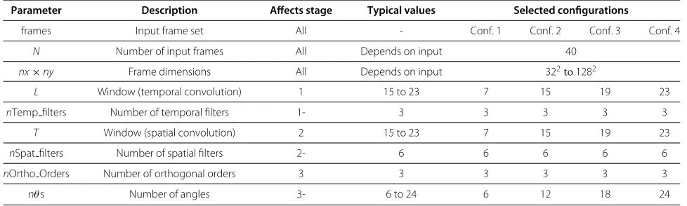
Evaluating the performance of McGM is a hard task, mainly due to the large amount of parameters that can be modified in order to tune the algorithm behavior. Many of those parameters have a great impact not only on the precision of the solution but also on the over-all attained performance. Table 1 lists the main config-urable parameters associated with the first three stages of McGM. The column labeled as ‘Typical values’ provides an overview of the most common values, although dif-ferent ones can be used to vary the motion estimation accuracy.
In Table 1, we also add four different parameter con-figurations that will be used for global throughput eval-uation. Although all experimental results are reported for video sequences with square frames, our imple-mentation is prepared for non-squared images, and no qualitative differences in the performance results have been observed.
Table 1 Main parameters involved in the McGM algorithm
Parameter Description Affects stage Typical values Selected configurations
frames Input frame set All - Conf. 1 Conf. 2 Conf. 3 Conf. 4
N Number of input frames All Depends on input 40
nx×ny Frame dimensions All Depends on input 322to1282
L Window (temporal convolution) 1 15 to 23 7 15 19 23
nTemp filters Number of temporal filters 1- 3 3 3 3 3
T Window (spatial convolution) 2 15 to 23 7 15 19 23
nSpat filters Number of spatial filters 2- 6 6 6 6 6
nOrtho Orders Number of orthogonal orders 3 3 3 3 3 3
4.2 McGM implementation on the DSP
The main implementation details and optimization tech-niques applied in our McGM porting task to the multi-core DSP are detailed in this section. As exposed in the algorithm description, we will divide the overall procedure into stages, describing each one in detail. Many of the optimization techniques applied for the DSP are quite similar for all stages. Therefore, the common optimization techniques are explained in detail next.
1. Basic implementation. We establish a baseline C implementation for comparison purposes. It includes the necessary compiler optimization flags and common optimization techniques to avoid unnecessary calculations and benefit from data locality and cache hierarchy. No further DSP-specific optimizations are applied in the code of this naive implementation.
2. DMA and memory-hierarchy optimization. One of
the strengths of the DSP is the ability of explicitly managing on-chip memory levels (L1 cache, L2 cache, and MSMC memory). Thus, one can define buffers, assign them to a particular
memory-hierarchy level (using the appropriate
#pragmaannotations in the code), and perform data copies between them as necessary. In addition, DMA capabilities are offered in order to overlap data transfers between memory levels and computation.
The usage of blocking and double-buffering is required. This involves the allocation of the current block of each frame to be processed and the next block which is being transferred through DMA while CPU computation is in progress. This technique effectively hides memory latencies, improving the overall throughput. In our case, we have mapped the temporal buffers that accommodate blocks of the input frames to the on-chip MSMC memory, in order to improve memory throughput in the computation stage.
3. Loop optimization. VLIW architectures require a careful loop optimization in order to let the compiler effectively apply techniques such as software pipelining, loop unrolling, and data prefetching [26]. In general, the aim is to keep the (eight) functional units of the core fully occupied as long as possible. To achieve this goal, the developer guides the compiler about safe loop unrolling factors, fixed
unroll counts (using appropriate#pragma
constructions), or pointer disambiguation (using
restrictkeyword on those pointers that will not overlap during the computation) by means of the mentioned tags orpragmas. Even though this type of optimizations is not critical in superscalar processors that defer the extraction of instruction-level
parallelism to execution time, it becomes crucial for VLIW architectures, even more for algorithms heavily based on loops as McGM. We have performed a full search to find the optimal unroll factor for each loop in the algorithm.
4. SIMD vectorization. As mentioned in Section 3, each C66x core is able to execute single-cycle arithmetic and load/store instructions on vector registers up to 128-bit wide. Naturally, this feature is supported at ISA level and can be programmed using intrinsics [26]. In McGM, data parallelism is massive and can be exploited by means of SIMD instructions in many scenarios. Intermediate data structures are stored using single-precision floating point (32-bit wide).
Thus, in the convolution step, input data can be grouped and processed in a SIMD fashion using 128-bit registers (usually referred asquad registers) for multiplications and 64-bit registers for additions. Given that the C66x architecture can execute up to eight SP multiplications (four per each M unit) and eight SP additions (two per each L and S unit), each core can potentially execute up to eight SP
multiplication-additions per cycle if SIMD is
correctly exploited. At this stage, we load and operate on four consecutive pixels of the image, unrolling the corresponding loop by a factor 4. Special caution must be taken in order to meet the memory alignment restrictions of the load/store vector instructions; to meet them, we apply zero-padding to the input image when necessary, according to its specific dimensions.
5. Loop parallelization. Up to this point, all the optimizations have been focused on exploiting parallelism at core level. The last stage of the
optimization involves the exploitation of thread-level parallelism to leverage the multiple cores in the DSP. The parallelization is carried out by means of OpenMP. Special care must be taken with shared variables, as no cache coherence is automatically maintained. Thus, data structures must be
zero-padded to fill a complete cache line and to avoid false sharing, and explicit cache write-back and/or invalidate operations must be performed in order to keep coherence between local memories to each core.
4.2.1 Stage 1: temporal filtering
Algorithm and implementation In order to obtain the temporal derivative of the image, it is necessary to per-form a convolution of each image sequence with each one of the three temporal filters obtained (low-passand two band-passfilters.)
necessary, prior to computation. As the number of tem-poral filters usually remains constant and is reduced (i.e., nTemp filters = 3), performance rates of this stage greatly depend on the window size (L) in which we apply the temporal filters and on frame dimensions (nx×ny).
Algorithm 1 temp filt = stage I (frames, N, L, nTemp filters,α,τ)
fortf = 0 tonTemp filtersdo
T filters (tf ) = get temporal filter (α,τ){Get filters} forfr = 0≤N−Ldo
frame = framesin(fr) for allp= pixel∈framedo
temp filt[tf ][p]←[p∗T filters]{Convolvep⊗ T filters}
end for end for end for
As output,nTemp filters matrices of the same dimen-sions as each input frame are generated as a result of the convolution of each frame with the corresponding con-volution filter. These matrices will be the input for the second stage (spatial filtering.)
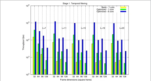
DSP optimizations and performance results Figure 4 reports the experimental results obtained after the imple-mentation and optimization of the temporal filtering
stage. Throughput results are given in terms of frames per second, considering increasing square frame dimensions and increasing window sizes (L) for the temporal convo-lution. We do not report results for a different number of temporal filters, as three is the most common configura-tion for McGM. We compare the throughput attained by the basic implementation using one core, with that of a version with all the exposed optimizations applied on one core, and parallelized across the eight available cores in the C6678.
At this stage, the critical factors affecting performance are frame size (nx×ny) and temporal window size (L). In general, for a fixedL, throughput decreases for increas-ing frame dimensions. For a fixed frame dimension, the impact of increasing the window size is also translated into a decrease in performance, although not in a relevant factor.
Independently from the evaluated frame resolution and window dimensions, core-level optimizations (usage of DMA, loop optimizations, and SIMD vectorization) are translated into performance improvements between ×1.5 and×2, depending on the specific selected param-eters. When OpenMP parallelization is applied, the
throughput improvement yields between ×5.5 and ×7
compared with the optimized sequential version. In gen-eral, the throughput obtained by applying the com-plete set of optimizations improves the original basic
implementation in a factor between ×7 and ×14. We
would like to remark the multiplicative effects observed
102 103 104 105 106
32 64 96 128 32 64 96 128 32 64 96 128 32 64 96 128 32 64 96 128
Throughput (fps)
Frame dimensions (square frame) Stage 1. Temporal filtering
Basic - 1 core Optimized - 1 core Optimized - 8 core
L=7 L=11 L=15 L=19 L=23
when both in-core and multi-core optimizations are carried out.
4.2.2 Stage 2: spatial filtering
Algorithm and implementation From the algorithmic point of view, spatial filtering does not dramatically dif-fer from the previous stage, see Algorithm 2. For each one of the spatial filters generated a priori and each one of the temporal-filtered frames, we apply a bi-dimensional convolution. Note that the amount of gen-erated data increases compared with that received from the previous stage in a factor of nSpat filters. The win-dow size in the convolution (T parameter) is the key in terms of precision and performance. As a result of this stage, we obtain a set of intermediate spatially filtered frames that will be provided as an input to the steering stage.
Algorithm 2 spat filt = stage II (temp filt, N, L, nTemp filters,nSpat filters,T)
forsf = 0 tonSpat filtersdo
S filt[sf ] =get spatial filter (sf ) {Get filters} end for
fortf = tonTemp filtersdo forfr = 0≤N−Ldo
frame = framesin(fr) for all p= pixel∈framedo
forsf = 0 tonSpat filtersdo
spat filt[sf ][tf ][p]←conv2D(temp filt[tf ][p], S filters(sf ),T)
end for end for end for end for
DSP optimizations and performance results Besides the basic implementation derived from the algorithmic definition of the stage, our optimizations (loop optimiza-tion, vectorization, and parallelization) are focused on the bi-dimensional convolution kernel in order to adapt it to DSP architecture specifications. More specifically, we leverage the separability of the bi-dimensional convolu-tion to perform and highly optimize one-dimensional (1D) vertical and horizontal convolutions, applying optimiza-tions at instruction level (loop unrolling), data level (vec-torization in the 1D convolution loop body), and thread level across cores (through OpenMP).
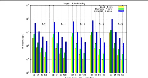
Figure 5 reports the experimental results obtained after the implementation and optimization of the spatial fil-tering stage. Results are presented for different frame dimensions and increasing spatial window sizes. As pre-vious considerations for the temporal stage, a comparison between a baseline version, an in-core-level optimization,
and optimized version across multi-core has also been performed.
At this stage, frame size (nx×ny) and spatial window size (T) substantially impact performance rates. As for the previous stage, when fixing T, throughput decreases for increasing frame dimensions. However, for a fixed frame dimension, the impact of increasing the spatial win-dow size is translated into higher throughput; from our analysis, our separate bi-dimensional convolution imple-mentations attain better performance as window size increases, mainly due to the avoidance of memory latency effects. This improvement, though, is expected to stabilize for larger window sizes (that are usually not common in McGM).
Core-level optimizations are translated into perfor-mance improvements between×1.6 and×2.2, depending on the evaluated frame and window dimensions. The thread-level parallelization yields an improvement bet-ween×5 and×6.5 when comparing with the optimized sequential version. In general, the throughput obtained by applying the complete set of core-level optimizations and thread-level parallelization improves the original basic implementation in a factor between×8 and×13.
4.2.3 Stage 3: steering filtering
Algorithm and implementation Algorithm 3 describes the necessary steps to perform the steering stage in the McGM method. Basically, the algorithm proceeds by applying a convolution between each spatial-filtered frame obtained from the previous stage (I in the algo-rithm), and an oriented filterFθpreviously calculated. The response of each one of the temporal- and spatial-filtered frames to this oriented filter will be the output of this stage.
Algorithm 3R= stage III (spac filt,N,L,nTemp filters, nSpat filters,nOrtho Orders,nθs )
forθ =0 tonθsdo
foroo = 0 tonOrtho Ordersdo forsf = 0 tonSpat filtersdo
fortf = 0 tonTemp filtersdo forfr = 0≤N−Ldo
frame = framesin(fr) for all p= pixel∈framedo
I= spat filt[sf ][tf ][p]
Rθ[oo][sf ][tf ][p] ←[Fθ ∗I] {Convolve F⊗I}
100 101 102 103 104 105
32 64 96 128 32 64 96 128 32 64 96 128 32 64 96 128 32 64 96 128
Throughput (fps)
Frame dimensions (square frame) Stage 2. Spatial filtering
Basic - 1 core Optimized - 1 core Optimized - 8 cores
T=7 T=11 T=15 T=19 T=23
Figure 5Throughput of the DSP implementation of the spatial filtering stage.For different frame dimensions and spatial window sizes.
DSP optimizations and performance results The opti-mizations applied to this stage are in the same way as those presented from the previous stages. Data paral-lelism is heavily exploited when possible, and loops are optimized after a deep search of the optimal unrolling parameters. OpenMP is used to extract thread-level par-allelism and leverage the power of the eight cores in the C6678.
Special caution must be taken at this stage with mem-ory consumption, as it reaches the maximum memmem-ory requirements of the McGM algorithm. More specifically, at this point, both the spatial-filtered frames and their steering filtering must coexist in the memory. However, this potential issue is conditioned by input algorithm parameters which are known beforehand.
Figure 6 reports the experimental results obtained after the implementation and optimization of the steering stage. Results are presented for different frame dimen-sions and different number of angles (orientations). As in previous stages, we compare the throughput attained by the basic implementation with that of a version with all the exposed core-level optimizations applied on one core, and with these optimizations together when the computation is distributed across eight cores.
At this stage, the factors affecting performance are frame size (nx× ny) and number of orientations (nθs). For a fixed number of angles, throughput decreases for increasing frame dimensions. For a common resolution, increasing the number of angles considered also yields
higher throughput. Core-level optimizations are more significant here, being the reason the higher arithmetic intensity in the loop bodies. These optimizations yield performance improvements between×4 and×5, depend-ing on the evaluated frame dimensions and number of angles. The thread-level parallelization yields an improve-ment between ×1.5 and ×2.5 taking as a reference the optimized sequential version, with higher improvements as the number of orientations is increased. In general, the throughput obtained by applying the complete set of optimizations outperforms the basic implementation in a factor between×10 and×12.5.
4.2.4 Final stages
10-1 100 101 102 103
32 64 96 128 32 64 96 128 32 64 96 128 32 64 96 128
Throughput (fps)
Frame dimensions (square frame) Stage 3. Steering
Basic - 1 core Optimized - 1 core Optimized - 8 core
nθs=6 nθs=12 nθs=18 nθs=24
Figure 6Throughput of the DSP implementation of the steering stage.For different frame dimensions and number of angles.
0 20 40 60 80 100 120
32 64 96 128
Time percentage
Frame dimensions (square frame) Stage time decomposition for McGM
Stage 1 Stage 2 Stage 3 Final stages
Table 2 Throughput of the DSP implementation of McGM for different parameter configurations
Throughput (fps)
322 642 962 1282
Conf. 1 266.86 60.34 25.78 14.18
Conf. 2 343.15 54.83 21.39 11.27
Conf. 3 503.27 54.99 11.77 9.89
Conf. 4 650.71 57.48 19.45 9.79
4.3 Global throughput results and real-time considerations
Besides the isolated throughput attained by each individ-ual stage of the algorithm analyzed in detail in previous sections, an overall view of the performance attained by the complete pipeline execution is necessary. Table 2 reports the throughput, in terms of frames per second, of the complete McGM implementation, considering only the most optimized version of each stage. Due to the wide variety of parameter combinations in the algorithm, we have chosen four different representative configura-tions, labeled as ‘Conf. 1 to Conf. 4,’ whose parameters are detailed in Table 1. Results are provided for increasing frame resolutions.
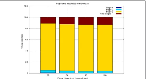
In general, throughput is reduced for increasing frame resolutions. While this rate is high for the minimum tested resolution (up to 650 fps for 32×32 frames), it dramat-ically decreases for larger frames, achieving a minimum of 9.74 fps for the largest resolution tested (128× 128). Differences between several parameter configurations are specially significant for small frame dimensions but not critical for the rest. Comparing the global performance results with those for each one of the stages presented in Figures 4, 5, and 6, the main insight is that the steer-ing stage is the clear limiting factor. Global throughput
is far from that attained in the temporal and
spa-tialfiltering stages (that were in the order of thousands of frames per second, depending on the resolution) and
closer to that attained for thesteeringstage. This confirms the time breakdown detailed in Figure 7, which illus-trates that 90% of the overall execution time is devoted to this stage.
In order to put results into perspective, Table 3 com-pares the throughput (in terms of frames per second) for a collection of platforms representative of current multi-core technology. We have selected a high-end general-purpose processor (Intel Xeon) and two different architectures as representatives of current low-power solutions, namely:
- TI DSP C6678 processor (eight cores) at 1 GHz with 512 Mbytes of RAM.
- Two Intel Xeon X5570 (eight cores in two sockets) at 2.93 GHz with 24 Gbytes of RAM.
- Intel Atom D510 (two cores) at 1.66 GHz with 2 Gbytes of RAM.
- ARM Cortex A9 (two cores) at 1 GHz (built by TI) with 1 Gbyte of RAM.
The table also reports the TDP in order to give an overview of the peak power consumption for each one of the platforms. Note that the TI C6678 DSP can be con-sidered as a low-power architecture, especially compared with the Intel Xeon (10 vs. 190 W when the two sockets of the latter are used). However, it is still far from the reduced power dissipated by the ARM Cortex A9.
Clearly, the multi-threaded implementation of McGM on the eight cores of the Intel Xeon yields the highest throughput rate from all the evaluated frame dimensions. For input images of 128×128 pixels, the throughput rate is roughly 21 fps. When only one core of the Intel Xeon is used, this rate is reduced to 4 fps. Our optimized imple-mentation on the C6678 DSP outperforms the sequential results on the Intel Xeon, achieving a peak rate for the largest tested frame dimensions of 9.74 fps. Consider-ing a rate around 20 fps, acceptable for beConsider-ing consid-ered as real-time processing (performance rates meeting real-time processing are in italic in Table 3), the parallel
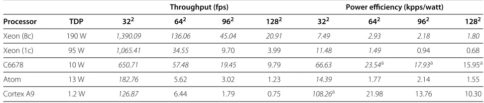
Table 3 Throughput and power efficiency of McGM implementations on different architectures, using Conf. 4 and different frame sizes
Throughput (fps) Power efficiency (kpps/watt)
Processor TDP 322 642 962 1282 322 642 962 1282
Xeon (8c) 190 W 1,390.09 136.06 45.04 20.91 7.49 2.93 2.18 1.80
Xeon (1c) 95 W 1,065.41 34.55 9.70 3.99 11.48 1.49 0.94 0.68
C6678 10 W 650.71 57.48 19.45 9.79 66.63 23.54a 17.93a 15.95a
Atom 13 W 182.76 5.62 3.02 1.23 14.39 1.77 2.14 1.55
Cortex A9 1.2 W 126.87 6.44 1.79 0.75 108.26a 21.98 13.76 10.30
implementation on the Intel Xeon can attain real-time on resolutions up to 128×128, meanwhile the TI DSP can attain real-time processing on up to 96×96 frame dimen-sions. Given the scalability observations extracted from our experimental results, we do not observe any relevant limitation for better performance results in future multi-core DSP architectures, possibly equipped with a larger number of cores.
4.4 Power efficiency considerations
This throughput rates must be considered in the context of the real power dissipated by each platform. To illus-trate the power efficiency of each platform when execut-ing McGM, Table 3 also provides a comparative analysis of the efficiency of each architecture in terms of thou-sands of pixels processed per second (kpps) per watt. The best power efficiency ratios are indicated with superscript letters in the table. Note that even though the ultra-low-power ARM is the most efficient architecture for the smallest input images (32×32), the TI DSP is clearly the most efficient platform for larger images. In this sense, the TI DSP offers a trade-off between performance and power that can be of wide appeal for those applications and sce-narios in which power consumption is a restriction, but real time is still a requirement for medium/large image inputs.
General-purpose multi-core architectures deliver lower rates in terms of power efficiency but are a requirement if real-time processing is needed for the largest tested images. Compared with the other two low-power archi-tectures (Intel Atom and ARM Cortex A9), real-time pro-cessing is only achieved for low-resolution images (32×32 in both cases). Thus, our DSP implementation, and the DSP architecture itself, can be considered as an appealing architecture not only when low power is desired but also when throughput is a limiting requirement.
5 Conclusions
In this paper, we have presented a detailed performance study of an optimized implementation of a robust motion estimation algorithm based of a gradient model (McGM) on a low-power multi-core DSP. Our study reports a general description of each stage of the multi-channel algorithm, with several optimizations that offer appeal-ing throughput gains for a wide range of execution parameters.
We do not propose the TI DSP architecture as a replacement of high-end current architectures, like novel multi-core CPUs or many-core GPUs, but as an attrac-tive solution for scenarios with tight power-consumption requirements. DSPs allow trade-off between perfor-mance, precision, and power consumption, with clear gains compared with other low-power architectures in terms of throughput (fps). In particular, while real-time
processing is attained only for low-resolution image sequences on current low-power architectures
(typi-cally 32 × 32 frames), our implementations elevates
this condition up to images with resolution 96 × 96
or higher, depending on the inputs execution parame-ters. These results outperform those on a single core of a general-purpose processor and are highly competitive with optimized parallel versions in exchange of a dramatic reduction in power requirements.
These encouraging results open the chance to consider these architectures in mobile devices where power con-sumption is a severe limiting factor, but throughput is a requirement. Our power consumption considerations are based on estimated peak dissipated power as provided by manufactures in the processor specifications. Neverthe-less, to be more accurate in terms of power consumption, we will consider as future work a more detailed energy evaluation study, offering real measurements at both core and system level.
Competing interests
The authors declare that they have no competing interests.
Acknowledgements
This work has been supported by Spanish Projects CICYT-TIN 2008/508 and TIN2012-32180.
Received: 31 January 2013 Accepted: 10 April 2013 Published: 10 May 2013
References
1. CL Huang, YT Chen, Motion estimation method using a 3D steerable filter. Image Vision Comput.13(1), 21–32 (1995)
2. BD Lucas, T Kanade, inProc. of 7th Int. Joint Conf. on Artificial Intelligence (IJCAI ’81). An iterative image registration technique with an application to stereo vision (Morgan Kaufmann Publishers Inc, San Francisco, CA, USA, April 1981), pp. 674–679
3. H-S Oh, H-K Lee, Block-matching algorithm based on an adaptive reduction of the search area for motion estimation. Real-Time Imaging.
6, 407–414 (October 2000)
4. D Sun, JP Lewis, Michaelj, inProc. ECCV. Black. Learning optical flow (Brown University, Providence, Rhode Island 02912, USA, 2008), pp. 83–97 5. S Baker, R Gross, I Matthews, Lucas-kanade 20 years on: a unifying
framework: part 3. Int J Comput Vis.56, 221–255 (2002)
6. X Liang, PW McOwan, A Johnston, Biologically inspired framework for spatial and spectral velocity estimations. J. Opt. Soc. Am. A.28(4), 713–723 (April 2011)
7. CP Benton, PW McOwan, A Johnston, Robust velocity computation from a biologically motivated model of motion perception. Proc R Soc B.
266, 509–518 (1999)
8. A Johnston, CW Clifford, A unified account of three apparent motion illusions. Vision Res.35(8), 1109–1123 (April 1995)
9. F Ayuso, G Botella, C Garcia, M Prieto, F Tirado, GPU-based acceleration of bio-inspired motion estimation model. Concurrency and Computation: Practice and Experience, In press
10. GB Juan, R´ıos Garc´ıa A, M Rodriguez-Alvarez, ER Vidal, U Meyer-B¨ase, MC Molina, Robust bioinspired architecture for optical-flow computation. IEEE Trans. VLSI Syst.18(4), 616–629 (2010)
11. C Dhoot, VJ Mooney, SR Chowdhury, LP Chau, inVLSI-SoC. Fault tolerant design for low power hierarchical search motion estimation algorithms (IEEE Computer Society, Los Alamitos, CA (USA), 2011), pp. 266–271 12. Vleeschouwer De C, T Nilsson, inICIP (2). Motion estimation for low power
13. M Anguita, J D´ıaz, E Ros, FJ Fernandez-Baldomero, Optimization strategies for high-performance computing of optical-flow in general-purpose processors. IEEE Trans. Circuits Syst. Video Techn.19(10), 1475–1488 (2009) 14. D Honegger, P Greisen, L Meier, P Tanskanen, M Pollefeys. IROS (IEEE,
2012), pp. 5177–5182
15. B Subramaniam, Wu-chun Feng, in8th IEEE Workshop on
High-Performance, Power-Aware Computing (HPPAC). The Green Index: A Metric for Evaluating System-Wide Energy Efficiency in HPC Systems (IEEE Computer Society, Los Alamitos, CA (USA), May 2012)
16. Y Shirai, J Miura, Y Mae, M Shiohara, H Egawa, S Sasaki, inComputer Architectures for Machine Perception, 1993. Proceedings. Moving object perception and tracking by use of dsp (IEEE Computer Society, Los Alamitos, CA (USA), Dec 1993), pp. 251–256
17. BKP Horn, BG Schunck, Determining optical flow. Artif. Intell.17, 185–203 (1981)
18. T Rwekamp, M Platzner, L Peters, inIn Proceedings of the 8th ICSPAT. Specialized architectures for optical flow computation: A performance comparison of asic, dsp, and multi-dsp, (1997), pp. 829–833
19. A Steimer, inMaster Thesis. ETH Zurich. Global optical flow estimation by linear interpolation algorithm on a DSP microcontroller, (Switzerland, October, 2011)
20. MV Srinivasan, An image-interpolation technique for the computation of optic flow and egomotion. Biol. Cybernetics.71, 401–415 (1994) 21. RJ Snowden, RF Hess, Temporal frequency filters in the human peripheral
visual field. Vision Res.32(1), 61–72 (1992)
22. JJ Koenderink, Optic flow. Vision Res.26, 161–180 (1996) 23. TMS320C6678 Multicore Fixed and Floating-Point Digital Signal
Processor. http://www.ti.com/lit/ds/sprs691c/sprs691c.pdf, February 2012. Texas Instruments Literature Number: SPRS691C
24. F Ayuso, G Botella, C Garcia, M Prieto, F Tirado, inWPABA 2011. GPU-based acceleration of bioinspired motion estimation model (IEEE Computer Society Washington, DC, USA, 2011)
25. F Ayuso, G Botella, C Garcia, M Prieto, F Tirado, in21st Int. Conf. on Field Programmable Logic and Applications, Workshop on Computer Vision on Low-Power Reconfigurable Architectures, 2011. GPU-based signal processing scheme for bioinspired optical flow (IEEE Computer Society, Los Alamitos, CA (USA), p. 2011. 09/2011 (2011)
26. Introduction to TMS320C6000 DSP optimization. http://www.ti.com/lit/ an/sprabf2/sprabf2.pdf, October 2011. Texas Instruments Literature Number: SPRABF2
doi:10.1186/1687-6180-2013-99
Cite this article as: Igual et al.: Robust motion estimation on a low-power multi-core DSP.EURASIP Journal on Advances in Signal Processing2013 2013:99.
Submit your manuscript to a
journal and benefi t from:
7Convenient online submission 7Rigorous peer review
7Immediate publication on acceptance 7Open access: articles freely available online 7High visibility within the fi eld
7Retaining the copyright to your article

![Figure 3 Functional diagram of the C66x DSP core architecture (source: [23]).](https://thumb-us.123doks.com/thumbv2/123dok_us/903286.1108992/6.595.57.541.429.715/figure-functional-diagram-c-dsp-core-architecture-source.webp)