Interference alignment schemes for k user interference channel based on manifold optimization

R E S E A R C H

Open Access

Interference alignment schemes for

k

-user interference channel based on

manifold optimization

Chen Zhang

, Ziwei Liu

, Tao Hong

and Gengxin Zhang

Abstract

Interference alignment (IA) is a key technology for achieving the capacity scaling required by next generation wireless networks, which is proved to obtain the maximum degrees of freedom (DoF). The aim of this paper is to propose

interference alignment schemes through manifold optimization theory forK-user interference channel. We limit the

optimization only at transmitters and relax the hypothesis of channel reciprocity to mitigate the overhead caused by alternation between the forward and reverse links significantly. Firstly, we introduce a classical algorithm based on the steepest descent (SD) algorithm in a multi-dimensional complex space to achieve feasible IA. Then, we reform the optimization problem on Stiefel manifold and propose a novel SD algorithm based on this manifold with lower dimensions. Moreover, aiming at further reducing the complexity, the Grassmann manifold is introduced to derive corresponding algorithm for reaching the perfect IA. Numerical simulations show that the proposed algorithms on manifolds have better performance both on system throughput and convergence than classical methods and also achieve the maximum DoF.

Keywords: Interference alignment, MIMO, Precoding, Manifold, Optimization

1 Introduction

Interference alignment (IA) has been envisioned as a promising technique [1, 2] to meet the overwhelming growth of data network traffic which is the main challenge of the next wireless networks. Compared with what is pre-viously believed, it can obtain even more higher network capacity [3]. Generally speaking, there are three domi-nant interference alignment schemes: The first scheme is based on full channel state information (CSI), assuming the transmitters have the priori perfect CSI; the second one is based on limited (imperfect) CSI; and the third one do not need the CSI, which is called blind interference alignment. Except for the full CSI interference alignment scheme, the other schemes have no complete degrees of freedom (DoF) region even the total DoF for theK-user

*Correspondence:[email protected]

1_{National Engineering Research Center of Communication and Network} Technology, Nanjing University of Posts and Telecommunications, Nanjing 210003, People’s Republic of China

2_{College of Telecommunications and Information Engineering, Nanjing} University of Posts and Telecommunications, Nanjing 210003, People’s Republic of China

interference channel [4,5], thus the feasibility of imperfect CSI interference alignment and blind interference align-ment is still an open problem. Consequently, in this paper, we focus on the full CSI interference alignment scheme. And the sum capacity ofK-userM× Mmultiple-input multiple-output (MIMO) interference channel is

Csum= KM

2 log(1+SNR)+o(log(SNR)) (1) where degrees of freedom (DoF) is defined as

DoF= lim

SNR→∞ Csum

log(SNR) (2)

In this case, DoF isKM/2. It means each transmitter-receiver pair can communicate withM/2 DoF, irrespec-tive of the number of interferers.

A feasible scheme to align interference is to design such a precoding that coordinates transmitting directions, for the purpose that the interference is forced to overlap as much as possible, and 1/2 signaling space is reserved for the desired signals at most. Based on the channel reci-procity’s assumption, some pioneer studies such as [6–10] iteratively optimize both the precoding matrices and

interference suppression filters, by alternating between the uplinks and downlinks to align the interference in a distributed way. However, with the hypothesis of chan-nel reciprocity, the application of these algorithms are only restricted within TDD systems. Moreover, at each node tight synchronization and feedback are needed for alternation between the downlinks and uplinks; when the channel varies fast, it may introduce too much overhead. Moreover, during each iteration process of optimization the transmitters and receivers exchange their “roles.” Thus this scheme is improper for the receivers with limited ability of computing.

On the other hand, most of the previous works above employ traditional constrained optimization techniques that work in high dimensional complex space. Unavoid-ably, several shortcomings are accompanied with the traditional constrained optimization techniques such as low-converging speed and high-complexity.

To overcome these limitations, in this paper, we intro-duce optimization on matrix manifolds into the precoding scheme for interference alignment and limit the optimiza-tion only at the transmitters’ side. Optimizaoptimiza-tion n on man-ifolds consist the merits of lower complexity and better numerical properties. Firstly, for the sake of comparison, by employing classical constrained optimization method, a steepest descent (SD) algorithm in multi-dimensional complex space is provided to design the precoder of interference alignment. Then, we reformulate the con-strained optimization problem to an unconcon-strained and non-degraded one on the complex Stiefel manifold with lower dimensions. We locally parameterize the manifold by Euclidean projection from the tangent space onto the manifold instead of the traditional method by moving descent step along the geodesic in [11,12]. Thus, the SD algorithm on Stiefel manifold is proposed to achieve fea-sible interference alignment. To further reduce the com-putation complexity in terms of dimensions of manifold, we explore the unitary invariance property of our cost function and solve the optimization problem on the com-plex Grassmann manifold, then present the corresponding SD algorithm on the Grassmann manifold for interference alignment precoding design.

We not only generalize optimization algorithm on manifolds, but also turn the algorithm into an efficient numerical procedure to achieve perfect interference align-ment. Moreover, by limiting the optimization algorithms performed at the transmitters’ side only, all the three proposed algorithms are transparent at the receivers. Additionally, overhead generated by synchronization and feedback no longer exists since only transmitters partici-pate in the iteration. Furthermore, by relaxing the assump-tion of channel reciprocity, our algorithms are applicable to both TDD and FDD systems. Furthermore, numerical simulation shows that the novel algorithms on manifolds

have better convergence performance and higher system capacity than previous methods. Finally, we prove the convergence of the proposed algorithms.

The paper is organized as follows: System model of interference alignment is presented in Section2, followed by the detailed procedures of all three proposed SD meth-ods for interference alignment in Section3. In Section4, numerical simulations and the corresponding discussion are stated. And the conclusion is given in the last section.

Notation: We use bold uppercase letters for matrices or vectors.XT andX†denote the transpose and the conju-gate transpose (Hermitian) of the matrixX, respectively. Assuming the eigenvalues of a matrix X and their cor-responding eigenvectors are sorted in ascending order,

λi

X denotes the ith eigenvalue of the matrix X. Then, I

represents the identity matrix. Moreover, tr(·) indicates the trace operation. And the Euclidean norm of X is

X = tr(X†X).Xdenotes the subspace spanned by the columns ofX.Cn×p_{represents then×pdimensional}

complex space assuming n > p.R+ represents positive real number space.{·}and{·}denote the real and imag-inary parts of a complex quantity, respectively. Finallyκ =

{1,. . .,K}is the set of integers from 1 toK.

2 System model

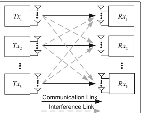
Consider the K-user wireless MIMO interference chan-nel depicted in Fig.1where each transmitter and receiver are equipped with M[k] andN[k] antennas, respectively. Each transmitter communicates with its corresponding receiver and creates interference to all the other receivers. d[k] is the desired number of data streams between the kth transmitter-receiver pair. Additionally, H[kj] denotes the N[k]× M[j] channel coefficients matrix from the jth transmitter to thekth_{receiver and is assumed to have i.i.d.}

1

Tx

Rx

2

Rx

k

Rx

Tx

k

Tx

complex Gaussian random variables, drawn from a con-tinuous distribution. Moreover,H is prior known at the transmitters. Finally the received signal vector at receiver kafter zero-forcing the interference is denoted by

Y[k]=U[k]†Y[k]=U[k]† sents an independently encoded Gaussian symbol with powerP[j]/d[j] that beamformed with the corresponding M[j] × d[j] precoding matrixV[j] and then transmitted by the transmitterj. U[k] is theN[k] ×d[k] interference zero-forcing filter at the receiverk. AndW[k]is the i.i.d. complex Gaussian noise with zero mean unit variance.

2.1 Feasibility of interference alignment

The quality of alignment is measured by the interfer-ence power remaining in the intended signal subspace at each receiver. From [6], it can be obtained that the d[k]-dimensional received signal subspace that contains the least interference is the space spanned by the eigen-vectors corresponding to thed[k]-smallest eigenvalues of the interference covariance matrixQ[k]. Consequently, we try to minimize the sum of interference power spilled to the desired signal subspaces, by minimizing the sum of the absolute value of d[k]-smallest eigenvalues of the interference covariance matrix at each receiver to cre-ate d[k]-dimensional interference-free subspace for the desired signal.

2.2 Cost function

As previously stated, we try to minimize the sum of the d[k]_{-smallest eigenvalues (in absolute value) of the} inter-ference covariance matrix at each receiver over the set of precoding matrices V[1],. . .,V[K] [7]. Therefore, we define the cost function as follows:

min

is the interference covariance matrix at receiverk. With the assumption that all the eigenvalues are sorted in ascending order,λi

Q[k] represents theitheigenvalue of the corresponding interference covariance matrix Q[k]. And becauseQ[k]is a Hermitian matrix, all its eigenvalues are

real. Therefore, the cost functionf(V),f :Cn×p_→R+_is

built.

3 Methods on different topologies for

interference alignment

3.1 The steepest descent algorithm in complex space for iA

Since our cost function:f(V),f : Cn×p → R+ is differ-entiable, intuitively, the steepest descent method can be employed to make the cost function converge to a local optimal point efficiently. Therefore, we will first find the closed-form expression of the steepest descent direction inCn×p, then employ a property step size rule for each iteration.

As previously stated, the steepest descent method is tightly related to derivative and differentiation. In order to get the derivative off(V)overV, two Jacobian matrices blocks are employed as: partial differential relation of the cost function over the real and imaginary parts ofV[j], respectively. The detail of mathematical derivations can be found in [7,13]. Thus, the derivative off overV[j]is given by

D[_Vj]=D_R[j]+iD[_Ij]T (7) The inner product typically defined in the Euclidean multi-dimensional space is given as follows:

Z1,Z2 =tr

Z†₂Z1

(8)

Then, under the given inner product, the steepest descent direction is:

Rule (10) guarantees that the stepβ[j]_Z[j]_{will expressively} decrease the cost function, whereas (11) undertakes that the step 2β[j]Z[j] would not be a better choice. A direct procedure for acquiring a suitableβ[j]is to keep on dou-blingβ[j]until (11) no longer holds and then halvingβ[j] until it satisfies (10). It can be proved that suchβ[j]can always be found [15].

Consolidating all the ideas stated above, we present our algorithm in Algorithm 1. In Step 3 and Step 4, the Armijo step rule is performed to find a proper conver-gence step length. Generally speaking, Step 3 ensures the chosen stepβ[j]will significantly reduce the cost function while Step 4 preventsβ[j]from being too large that may miss the potential optimal point. The operatorgs(·)means Gram-Schmidt Orthogonalization [16] of a matrix, which guarantees the newly computed solutionV[j](orB₁[j],B[₂j] ) still satisfies the unitary constraint.

Discussion:

(i) The inner product and the gradient direction are defined in different topologies in [7]. However, it is considered to be inappropriate because the gradient is defined after the inner product is given only. In

Algorithm 1The Steepest Descent Algorithm in Complex Space for IA

Start with arbitrary precoding matrices V[1], ...,V[K], set

initial step sizeβ[j]=1 and begin iteration.

forj=1...K

(1) Compute the Jacobian matrixD[_Rj]andD[_Ij]

(2) Get the steepest descent direction

Z[j]= −D[_Vj]= −(D_R[j]+iD[_Ij])T

(3) ComputeB[₁j]=gs(V[j]+2β[j]Z[j]),

iff(V[1], ...,VK)−f(V[1], ...,V[j−1],B[₁j],V[j+1]...V[K])

≥β[j]_tr(Z[j]†_Z[j]_{), then setβ}[j]_:=2β[j]_{, repeat Step 3.}

(4) ComputeB[₂j]=gs(V[j]+β[j]Z[j]),

iff(V[1], ...,V[K])−f(V[1], ...,V[j−1],B[₂j],V[j+1]...V[K])

<1

2β[j]tr(Z[j]

†_Z[j]_{), then setβ}[j]_:= 1

2β[j], repeat Step 4.

(5)V[j]=gs(V[j]+β[j]Z[j])

(6) Continue till the cost functionf is sufficiently small.

other words, the inner product and the gradient direction must be defined in the same topology. Our proposed algorithm rectifies the topology flaw in [7] and thus avoids the risk of non-convergence. (ii) It can be concluded that Algorithm 1 belongs to the

classical optimization method [17], which means it works in multi-dimensional spaceCn×pwith the dimensions:

dim(Cn×p)=np (12)

Obviously, the algorithm complexity increases with the dimensions. As previous discussed, optimization algorithms on manifolds work in an embedded or quotient space whose dimension will be much smaller than that of classical constrained optimization methods. Thus, optimization algorithms on manifolds not only have lower complexity, but also perform better numerical properties. The

corresponding algorithms on manifolds will be stated for IA in the next two subsections.

3.2 The steepest descent algorithm on complex stiefel manifold for iA

Informally, a manifold is a space that is “modeled on” Euclidean space. It can be defined as a subset of Euclidean space which is locally the graph of a smooth function.

Conceptually, the simplest approach to optimize a dif-ferentiable function is to continuously translate a test point in the direction of the steepest descent on the con-straint set until one reaches a point where the gradient is equal to zero. However, there are two challenges for opti-mization on manifolds. First, in order to define algorithms on manifolds, these operations above must be translated into the language of differential geometry. Second, once the test point shifts along the steepest descent direc-tion, it must be retracted back to the manifold. There-fore, after reformulating the optimization problem on the Stiefel manifold, we introduce definitions about project operation and tangent space for retraction and gradient, respectively.

In many cases, the underlying symmetry property can be exploited to reformulate the problem as a non-degenerate optimization problem on manifolds associated with the original matrix representation. Thus, the con-straint condition V[j]†V[j] = I in the cost function (4) inspires us to solve the problem on the complex Stiefel manifold. The complex Stiefel manifold [16]St(n,p)is the set satisfying

St(n,p)= {X∈Cn×p:X†X=I} (13) St(n,p)naturally embeds inCn×p _{and inherits the usual}

topology ofCn×p_{. It is a compact manifold and from [18],}

dim(St(n,p))=np−1

2p(p+1) (14)

Another important definition is the projection. Assum-ingY ∈ Cn×pis a rank-pmatrix, the projection operator

πst(·):Cn×p→St(n,p)is given by

πst(Y)=arg min

X∈St(n,p)Y−X

2 ₍₁₅₎

It can be proved that there exists a unique solution ifY has full column rank [18]. From (15), it can be acquired that the projection of an arbitrary rank-pmatrixY onto the Stiefel manifold is defined to be the point on the Stiefel manifold closest toY in the Euclidean norm [19]. More-over, if the singular value decomposition (SVD) of Y is Y =UV†, then

to move away fromXasεincreases. The collection of such directionsYis called the normal space atXofSt(n,p)[18]. The tangent spaceTX(n,p)is defined to be the orthogonal

complement of the normal space, which can be roughly illustrated as Fig.2. And the mathematical expression of the tangent spaceTX(n,p)atX∈St(n,p)is defined by

Fig. 2Tangent space of Stiefel manifold

Obviously the steepest descent algorithm requires the computation of the gradient. As we previously emphasize, the gradient is only defined afterTX(n,p)is given an inner inner product, the steepest descent direction of the cost functionf(X)at the pointX∈St(n,p)is

Z=XD†_XX−DX (20)

whereDXis the derivative off(X).

The proposed SD algorithm on complex Stiefel mani-fold is presented in Algorithm 2. From (19) and (20), it can be easily obtained that the inner product needed for the Armijo step rule is

which is used in Step 4 and 5, and the steepest descent on Stiefel manifold of our cost function is

Z[j]=V[j]D_V[j]†V[j]−D[_Vj] (22) which is used in Step 3. Noticing that the project opera-tionπst(·)in Step 6 (Steps 4 and 5) guarantees the newly

computed solutionV[j] (orB₁[j], B[₂j] ) after iteration still satisfiesV[j]∈St(n,p). Using the method of SVD, we can easily compute the project operation. Discussion:

(i) As previous stated, the algorithms in [11,12] were performed by moving the descent step along the geodesic of the constrained surface within each iteration. A disadvantage of this method is the redundant computational cost for calculating the path of a geodesic. In this paper, we locally parameterize the manifold by Euclidean projection from the tangent space onto the manifold instead of moving along a geodesic, to achieve a modest reduction in the computational complexity of the algorithms.

Algorithm 2The Steepest Descent Algorithm on Com-plex Stiefel Manifold for IA

Start with arbitrary precoding matricesV[1], ...,V[K],

forj=1...K

(1) Compute the Jacobian matrixD[_Rj]andD[_Ij]

(2) Then get the derivative off:

D_V[j]=(D_R[j]+iD[_Ij])T

(3) Get the steepest descent direction

Z[j]=V[j]D_V[j]†V[j]−D[_Vj]

(7) Continue till the cost functionf is sufficiently small.

3.3 The steepest descent algorithm on complex grassmann manifold for iA

Notice that our cost functionf(V)satisfiesf(V U)=f(V) for any unitary matrixU. Because

Q[k](V U)=

which means that multiplying unitary matrixU does not change the eigenvalues and their corresponding eigenvec-tors of the interference covariance matrix at each receiver. Thus, our cost function f should be minimized on the

Grassmann manifold rather than on the Stiefel manifold. This is because the Grassmann manifold treatsVandV U as equivalent points, leading to a further reduction in the dimension of the optimization problem. Similar with the previous subsection, we firstly introduce the definition about the Grassmann manifold, then present the project operation and tangent space of Grassmann manifold for retraction and gradient, respectively.

The complex Grassmann manifoldGr(n,p)is defined to be the set of allp-dimensional complex subspaces ofCn×p. The Grassmann manifold can be thought as a quotient space of the Stiefel manifold:Gr(n,p) St(n,p)/St(p,p). Quotient space is more difficult to visualize, as it is not defined as a set of matrices; rather, each point of the quotient space is an equivalence class ofn×pmatrices.

However, we can understand quotient space in this way: assuming X ∈ St(n,p) is a point on the Stiefel manifold, the columns of X span an orthonormal basis for ap-dimensional quotient subspace. That is to say, if

Xdenotes the subspace spanned by the columns ofX, then X ∈ St(n,p) implies X ∈ Gr(n,p). Therefore, there is a one-to-one mapping between points on the Grassmann manifoldGr(n,p) and equivalence classes of St(n,p). From (14), it can be acquired that:

dim(Gr(n,p))=dim(St(n,p))−dim(St(p,p))

=p(n−p) (24)

LetY ∈Cn×pbe a rank-pmatrix. The projection oper-ator πgr(·) : Cn×p → Gr(n,p) onto the Grassmann

manifold is defined to be

πgr(Y)=

It also can be proved that there exists a unique solution if Y has full column rank [18]. From (25), it can be acquired that the projection of an arbitrary rank-pmatrixY onto the Grassmannn manifold is defined to be the subspace spanned by the point on the Stiefel manifold closest toY in the Euclidean norm. Furthermore, if the QR decom-position ofY isY = QR, the following equality holds:

πgr(Y)=QIn×p (26)

The proof of (26) also can be found in [16]. From (26), it is obvious thatπgr(Y)is the subspace spanned by the firstp

columns ofQ.

As discussed before, Grassmann manifold is a quotient space of the Stiefel manifold, thus its tangent space is a subspace of the Stiefel manifold’s tangent space [18]. IfX∈

Recall (18), the dimension of the tangent spaceTX(n,p) of the complex Grassmann manifold is:

dim(TX(n,p))=dim(TX(n,p))−dim(TX(p,p))

=p(2n−2p) (28)

Moreover, the inner product ofTX(n,p)is given by:

Z1,Z2 = {tr(Z2†Z1)}, Z1,Z2∈TX(n,p),

X∈St(n,p) (29)

The derivation of (29) can be found in [16]. Therefore, under the defined inner product, the steepest descent direction [16] of the cost functionf(X)at the pointX ∈

Gr(n,p)is:

Z= −(I−XX†)DX (30)

whereDXis the derivative off(X).

The proposed SD algorithm on the complex Grassmann manifold is presented in Algorithm 3. Similar with the previous proposed algorithms, the Armijo step rule is per-formed to find a proper convergence step length. From

Algorithm 3The Steepest Descent Algorithm on Com-plex Grassmann Manifold for IA

Start with arbitrary precoding matricesV[1], ...,V[K],

forj=1...K

(1) Compute the Jacobian matrixD[_Rj]andD[_Ij]

(2) Then get the derivative off:

D_V[j]=(D_R[j]+iD[_Ij])T

(3) Get the steepest descent direction

Z[j]= −(I−V[j]V[j]H)D[_Vj]

(4) ComputeB[₁j]=πgr(V[j]+2β[j]Z[j]),

iff(V[1], ...,VK)−f(V[1], ...,V[j−1],B[₁j],V[j+1]...V[K])≥

β[j]_tr(Z[j]H_Z[j]_{), then setβ}[j]_:=2β[j]_{, and repeat Step 4.}

(5) ComputeB[₂j]=πgr(V[j]+β[j]Z[j]),

iff(V[1], ...,V[K])−f(V[1], ...,V[j−1],B[₂j],V[j+1]...V[K]) <

1

2β[j]tr(Z[j]HZ[j]), then setβ[j]:=12β[j], and repeat Step 5.

(6)V[j]=πgr(V[j]+β[j]Z[j])

(7) Continue till the cost functionfis sufficiently small.

(29) and (30), it can be easily concluded that the inner product needed for the Armijo step rule is

Z[j],Z[j]

=tr

Z[j]†Z[j]

(31)

which is used in Step 4 and 5, and the steepest descent on Grassmann manifold of our cost function is

Z[j]= −

I−V[j]V[j]†

D[_Vj] (32)

which is used in Step 3. And the project operationπgr(·)

in Step 6 (Step 4, 5) retracts the newly computed solu-tion V[j] (or B₁[j], B[₂j]) back onto Grassmann manifold Gr(n,p). Using QR decomposition, we can easily compute the project operation.

Discussion:

(i) Comparingdim(Gr(n,p))=p(n−p)in (24) with

dim(St(n,p))=np−1₂p(p+1)in (14), a further dimension reduction can be observed. Similarly, from (28), we can see another advantage of using the Grassmann manifold rather than the Stiefel manifold which is thatTX(n,p)has onlyp(2n−2p)

dimensions, whereas tangent space ofSt(n,p)has

p(2n−p)dimensions. And from [20], it can be obtained that in our system model, if each

transceiver is equipped with same amount of antenna (M=N), then

K

k=1

d[k]=K·d= K·M

2 (33)

and

d= M

2 (34)

(ii) Recall (12), (14), and (24), we can get that ifM is large enough (M not only can represent the number of antennas each transceiver equipped, but also can refer to the number of time extension slots [1,20]), hence

dim(St(M,d)) dim"CM×d# ≈

3

4 (35)

which is a clear evidence for dimension-descension. And

dim(Gr(M,d)) dim"CM×d# =

1

2 (36)

holds for any integerM. (36) means that optimization on Grassmann manifold would reduce dimension further. The trend of dimension-descension can be roughly illustrated in Fig.3.

4 Numerical results and discussion

Without symbol extension, the feasible condition of k-user interference alignment [20] is given by:

n p n p

( , )

Gr n p

X

†

( , ) :

St n p

X X

I

Fig. 3Trend of dimension-descension

For satisfying feasibility and simple computation, we con-sider a 3-user 2×2 MIMO interference channel where the desired DoF per userd[j]is 1. All the algorithms are executed under the same scenario including randomly generated channel coefficients, initial precoding matrices, and convergence step length. We simulated the proposed three SD algorithms through 100 simulation realizations.

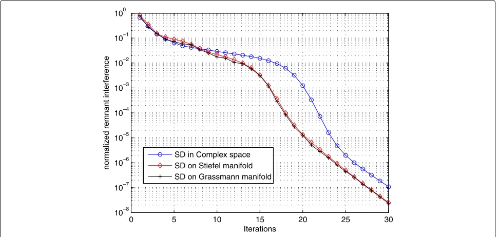
In order to compare the convergence performance, the average values of 100 realizations results are illus-trated in Fig. 4. It can be observed that the algorithms on manifolds have better convergence performance com-paring with the classical optimization method as our expectation.

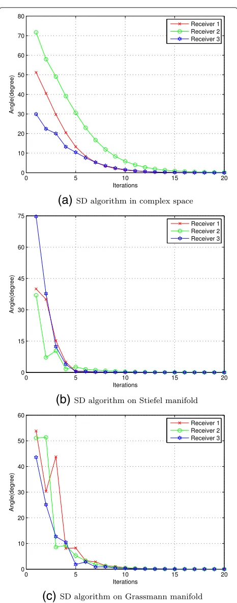
Meanwhile, since there are two interference sig-nals at each receiver, as shown in Fig. 5, the angles

between the spaces spanned by each interference signals asymptotically converge to zero within one simulation realization, which is another evidence for achieving the perfect interference alignment.

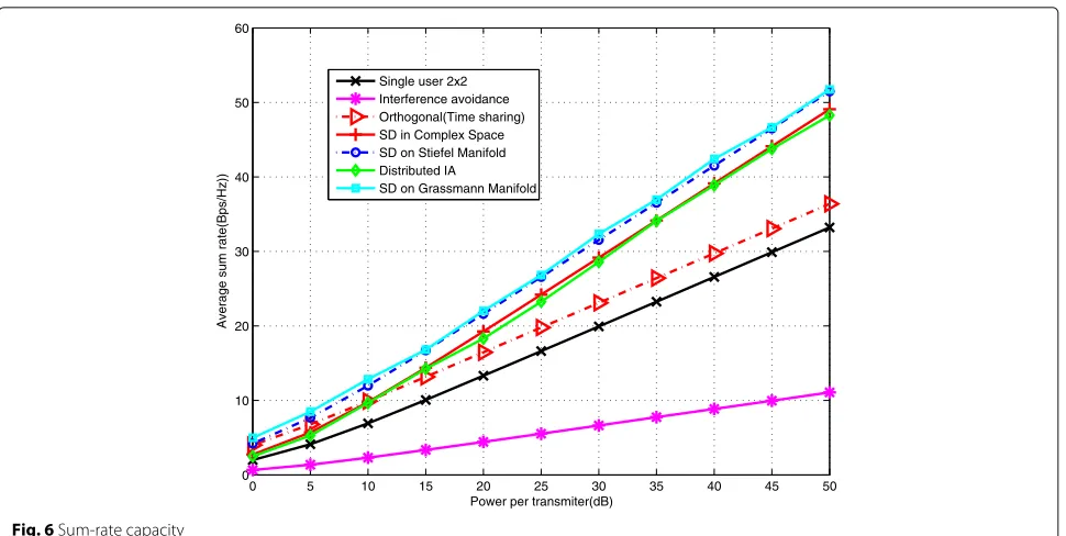
Finally, we compare the system sum-rate of the pro-posed algorithms. Figure 6shows that the SD algorithm on Stiefel manifold and the SD algorithm on Grassmann manifold almost have the same performance and out-perform the other classical optimization algorithms (Dis-tributed IA in [6,7]). More importantly, at high SNR, the DoF of the three proposed algorithms nearly achieve 3, which is the maximum theoretical value (KM/2 = 3) . Therefore, the perfect interference alignment is success-fully achieved.

Three reasons leading to the fact that the proposed algorithms on manifolds have better performance are pre-sented below:

(i) The advantage of the proposed algorithms is attributed to the reason that we reformulate the constrained optimization problem to an unconstrained one on manifolds with lower complexity and better numerical properties; then, locally parameterize the manifolds by a Euclidean projection of the tangent space on to the manifolds instead of moving along the geodesic, as stated in the previous sections. Moreover, the convergence performance curve of SD algorithm on the Stiefel manifold and the curve of SD algorithm on the Grassmann manifold almost overlap. Recall that optimization on the Grassmann manifold would reduce dimension further; therefore, the SD

0 5 10 15 20 25 30

10−8 10−7 10−6 10−5 10−4 10−3 10−2 10−1 100

Iterations

normalized remnant interference

SD in Complex space SD on Stiefel manifold SD on Grassmann manifold

(a)

(b)

(c)

Fig. 5Angles between interfering spaces at each receiver.aSD algorithm in complex space.bSD algorithm on Stiefel manifold.cSD algorithm on Grassmann manifold

algorithm on the Grassmann manifold will guarantee performance and reduce the computation

complexity at the same time.

(ii) It is noticed that our cost function actually is the interference power spilled from the interference space to the desired signal space. With the better convergence performance, the SD algorithms on manifolds will have less remnant interference in the desired signal space within same iteration times. Therefore, it’s guaranteed to achieve higher SINR [21]:

SINR= signal power

noise+remnant interference (38)

which leads to high capacity.

(iii) At each receiver, the zero-forcing filter is adopted. It will project the desired signal power and the remnant interference onto the subspace which is orthogonal with the subspace spanned by the interference. After performing the SD algorithms on manifolds, it is observed that in the Euclidean norm distance, the subspace spanned by desired signal is more close to the orthogonal complement of the interference subspace. Therefore, even the proposed algorithms on manifolds finally get the same remnant

interference as the classical optimization methods results. The algorithms on manifolds will suffer from less power lose during the projection operated by zero-forcing filter; hence, higher system capacity can be achieved.

Above all, we didn’t just correct the defects of our pre-vious results. More importantly, many innovations and improvements are made in this paper. Firstly, through the in-depth study of matrix manifold, many novel man-ifold conceptions (such as Stiefel manman-ifold, Grassmann manifold, quotient space, dimension decrease, and pro-jection) are introduced as the theoretical foundation to support reformulation of interference alignment objec-tive function on manifolds and also promote the pro-posed algorithms lower complexity, better convergence performance and higher system capacity. Secondly, from a self-contained system perspective, we cite part of our pre-vious result in Section3Algorithm 1 and propose novel algorithms on three different topologies (complex space, Stiefel manifold, and Grassmann manifold) for interfer-ence alignment. More importantly, we uniform the flow of the three proposed algorithms to make the compari-son of algorithms’ results become more meaningful and logicality.

0 5 10 15 20 25 30 35 40 45 50 0

10 20 30 40 50 60

Power per transmiter(dB)

Average sum rate(Bps/Hz))

Single user 2x2 Interference avoidance Orthogonal(Time sharing) SD in Complex Space SD on Stiefel Manifold Distributed IA

SD on Grassmann Manifold

Fig. 6Sum-rate capacity

Nevertheless, these methods to increase throughputs can be performed as the second step after the interference alignment is achieved. Thus in this paper, we only need to concentrate on the first step to find the perfect solutions of interference alignment.

More importantly, we notice that the limited CSI will give a disturbance to our algorithm [22–24]. However, its negative influence on our algorithm is tolerable due to three main reasons. First, the proof for the con-vergence of our proposed algorithm is solid: our cost function is non-negative with the low bound zero. It monotonically decreases within each iteration; there-fore, it must converge to a solution. Second, due to the property of steepest decent method, our algorithm will converge to a local optimum point even with a dis-turbance. Third, the numerical property of manifolds will guarantee the residual interference (the value of local optimum point) is very small which leads to high capacity.

5 Conclusion and future work

In this paper, we focus on the interference alignment schemes by employing manifold optimization theory. By restricting the optimization only at the transmitters’ side, the overhead induced by alternation between the forward and reverse links will be alleviated significantly. A classi-cal SD algorithm in multi-dimensional complex space is proposed first. Then, we reform the optimization problem on Stiefel manifold and propose a novel SD algorithm on this manifold with lower dimensions. Moreover, aiming at further reducing the complexity, the Grassmann manifold

is introduced to derive the corresponding algorithm for reaching the perfect interference alignment. Numerical simulations show that comparing with previous methods, the proposed algorithms on manifolds have better con-vergence performance, higher system capacity, and also achieve the maximum DoF.

In our future work, we will employ Newton-type method on manifolds to achieve quadratic convergence and try to find global optimum results. On the other hand, we already begin the research on Grassmannian dif-ferential quantization theory and deep-learning method [25] to offer a efficient feedback strategy for limited CSI interference alignment. This complicated work is still in progress.

Abbreviations

CSI: Channel state information; DoF: Degrees of freedom; FDD: Frequency division duplexing; IA: Interference alignment; MIMO: Multiple-input multiple-output; SD: Steepest descent; SNR: Signal-to-noise ratio; TDD: Time division duplexing

Acknowledgements

The authors would like to thank the reviewers for their helpful suggestions.

Authors’ contributions

CZ conceived the methods and wrote the paper. CZ and ZL analyzed the simulation data. GZ and TH gave valuable suggestions on the structure of the paper. ZL and TH revised the original manuscript. All authors read and approved the manuscript.

Funding

This work was supported by NUPTSF (Grant no. NY219121) and National Natural Science Foundation of China (Grant no. 91738201).

Availability of data and materials

Competing interests

The authors declare that they have no competing interests.

Received: 24 October 2018 Accepted: 18 July 2019

References

1. H. Maleki, V. R. Cadambe, S. A. Jafar, Index coding an interference alignment perspective. IEEE Trans. Inf. Theory.60(9), 5402–5432 (2014) 2. A. G. Davoodi, S. A. Jafar, Generalized degrees of freedom of the symmetric

k-user interference channel under finite precision CSIT. IEEE Trans. Inf. Theory.63(10), 6561–6572 (2017)

3. B. Yuan, H. Sun, S. A. Jafar, Replication-based outer bounds and the optimality of half the cake for rank-deficient MIMO interference networks. IEEE Trans. Inf. Theory.63(10), 6607–6621 (2017)

4. M. Morales-Cespedes, J. Plata-Chaves, D. Toumpakaris, S. A. Jafar, A. G. Armada, Cognitive blind interference alignment for macro-femto networks. IEEE Trans. Signal Process.65(19), 5121–5136 (2017) 5. A. G. Davoodi, S. A. Jafar, Transmitter cooperation under finite precision

CSIT: a GDoF perspective. IEEE Trans. Inf. Theory.63(9), 6020–6030 (2017) 6. K. S. Gomadam, V. R. Cadambe, S. A. Jafar, A distributed numerical

approach to interference alignment and applications to wireless interference networks. IEEE Trans. Inf. Theory.57(6), 3309–3322 (2011) 7. H. G. Ghauch, C. B. Papadias, inIEEE Global Telecommunications Conference

(GLOBECOM). Interference alignment: a one-sided approach (IEEE, Texas, 2011), pp. 1–5

8. J. Fanjul, O. Gonzalez, I. Santamaria, C. Beltran, Homotropy continuation for spatial interference alignment in arbitrary MIMO X networks. IEEE Trans. Signal Proc.65(7), 1752–1764 (2017)

9. S. M. Razavi, Unitary Beamformer designs for MIMO interference broadcast channels. IEEE Trans. Signal Process.64(8), 2090–2102 (2016)

10. H. Al-Shatri, X. Li, R. S. Ganesan, A. Klein, T. Weber, Maximizing the sum rate in cellular networks using multiconvex optimization. IEEE Trans. Wirel. Commun.15(5), 3199–3211 (2016)

11. S. Said, L. Bombrun, Y. Berthoumieu, J. H. Manton, Riemannian Gaussian distributions on the space of symmetric positive definite matrices. IEEE Trans. Inf. Theory.63(04), 2153–2170 (2017)

12. S. Said, H. Hajri, L. Bombrun, B. Vemuri, Gaussian distributions on Riemannian symmetric spaces statistical learning with structured covariance matrices. IEEE Trans. Inf. Theory.64(02), 757–772 (2018) 13. A. Hjorungnes,Complex-Valued Matrix Derivatives: With Applications in

Signal Processing and Communications. (Cambridge University Press, Cambridge, 2011), pp. 58–65

14. S. Boyd, L. Vandenberghe,Convex Optimization. (Cambridge University Press, Cambridge, 2004), pp. 437–489

15. E. Polak,Optimization: Algorithms and Consistent Approximations. (Springer-Verlag, Berlin, 1997), pp. 223–275

16. X. Zhang,Matrix Analysis and Applications. (Tsinghua University Press, Beijing, 2004), pp. 320–365

17. C. Zhang, H. Yin, G. Wei, inIEEE Vehicular Technology Conference (VTC Fall). One-sided precoder designs for interference alignment (IEEE, Quebec City, 2012), pp. 1–5

18. P. A. Absil, R. Mahony, R. Sepulchre. Optimization algorithms on matrix manifolds (Princeton University Press, New Jersey, 2008), pp. 53–69 19. K. Benidis, Y. Sun, P. Babu, D. P. Palomar, Orthogonal sparse PCA and

covariance estimation via procrustes reformulation. IEEE Trans. Signal Process.64(23), 6211–6226 (2016)

20. C. Wang, H. Sun, S. A. Jafar, Genie chains: exploring outer bounds on the degrees of freedom of MIMO interference networks. IEEE Trans. Inf. Theory.

62(10), 5573–5602 (2016)

21. Y. Cao, N. Zhao, F. R. Yu, M. Jin, Y. Chen, J. Tang, V. C. M. Leung, Optimization or alignment: secure primary transmission assisted by secondary networks. IEEE J. Sel. Areas Commun.36(4), 905–917 (2018) 22. C. Hao, B. Clerckx, Achievable sum DoF of the k-user MIMO interference

channel with delayed CSIT. IEEE Trans. Commun.64(10), 4165–4180 (2016) 23. M. Torrellas, A. Agustin, J. Vidal, Achievable DoF-delay trade-offs for the

k-user MIMO interference channel with delayed CSIT. IEEE Trans. Inf. Theory.62(12), 7030–7055 (2016)

24. S. Y. Yeh, I. H. Wang, Degrees of freedom of the bursty MIMO X channel without feedback. IEEE Trans. Inf. Theory.64(4), 2298–2320 (2018)

25. H. Huang, Y. Song, J. Yang, G. Gui, F. Adachi, Deep-learning-based millimeter-wave massive MIMO for hybrid precoding. IEEE Trans. Veh. Technol.68(3), 3027–3032 (2019)

Publisher’s Note