R E S E A R C H
Open Access
Performance analysis of
α
-
β
-
γ
tracking filters
using position and velocity measurements
Kenshi Saho
*and Masao Masugi
Abstract
This paper examines the performance of two position-velocity-measured (PVM)α-β-γtracking filters. The first estimates the target acceleration using the measured velocity, and the second, which is proposed for the first time in this paper, estimates acceleration using the measured position. To quantify the performance of these PVMα-β-γ filters, we analytically derive steady-state errors that assume that the target is moving with constant acceleration or jerk. With these performance indices, the optimal gains of the PVMα-β-γfilters are determined using a
minimum-variance filter criterion. The performance of each filter under these optimal gains is then analyzed and compared. Numerical analyses clarify the performance of the PVMα-β-γ filters and verify that their accuracy is better than that of the general position-only-measuredα-β-γfilter, even when the variance in velocity measurement noise is comparatively large. We identify the conditions under which the proposed PVMα-β-γfilter outperforms the generalα-β-γfilter for different ratios of noise variance in the velocity and position measurements. Finally, numerical simulations verify the effectiveness of the PVMα-β-γfilters for a realistic maneuvering target.
Keywords: α-β-γfilter; Moving target tracking; Position and velocity measurements; Steady-state error; Optimal gains; Minimum variance filter criterion
Introduction
Remote monitoring systems embedded in robots and vehicles require the capability to accurately track moving objects. Tracking filters, such as Kalman filters, extended Kalman filters (EKFs), and particle filters, are commonly used for this purpose [1-5]. These can accurately track movement based on adaptive filtering, which minimizes the error in the predicted position based on dynami-cal and measurement models. However, these techniques have a relatively heavy computational load, and in some cases their use is impractical. Moreover, their design is conducted empirically, because it is difficult to evaluate the validity of the design parameters (i.e., the process noise) [6,7].
One effective approach that does not suffer from these problems is known as anα-β-γ filter. These are simple tracking filters that assume constant acceleration during the sampling interval [8]. Because of their small computa-tional load, they have been employed in various tracking
*Correspondence: [email protected]
Department of Electronic and Computer Engineering, Ritsumeikan University, 1–1–1 Noji-Higashi, Kusatsu, Shiga 525-8577, Japan
systems [9-12]. Moreover, there are only three design parameters (theα,β, andγ gains), from which the per-formance indices can be analytically calculated. Conse-quently, it is simpler to design an appropriateα-β-γ filter than to construct other tracking filters (e.g., the Kalman filter). Many researchers have studied the analytical per-formance and design methodology of optimal gains in theα-β-γ filter by assuming simple and practical motion models [8,13-17]. Based on these fundamental studies, recent work has investigated effective gain-setting algo-rithms for various maneuvering targets [18,19]. Simple gain-setting algorithms have enabled the effectiveness of
α-β-γ filters to be verified in various real-world applica-tions, such as motor position control [9] and human fall detection [10].
Traditionally, tracking filter techniques have been applied to radar, sonar, and global positioning systems that measure position only [6]. However, various sensing sys-tems that can accurately measure velocity have recently been developed thanks to technical advances in various sensors and sensor networks, such as the micro-Doppler radar network [20,21]. Consequently, the application of tracking filters to such sensing systems has become an
important area of research [22-25]. We can expect mea-sured velocities to improve the accuracy of tracking com-pared with trackers that use position measurements alone. However, when the reliability of the velocity measure-ments is low, the tracking accuracy may deteriorate. Thus, the relationship between tracking accuracy and measure-ment noise is very important for the implemeasure-mentation of α-β-γ filters using both position and velocity mea-surements. Although position-velocity-measured (PVM) tracking filters have been investigated [23-28], the num-ber of such studies is quite small compared with those on general tracking filters that measure only position. Addi-tionally, most studies on PVM tracking filters use Kalman or particle filters. Several applications of PVMα-β-γ fil-ters have been reported [29,30], but these studies do not investigate the filters’ theoretical performance, meaning the tracking system parameters are designed empirically. Thus, their analytical properties have not been adequately investigated.
This paper analyzes PVM α-β-γ filters and compares their performance with that of a generalα-β-γ filter. For a fair comparison with the generalα-β-γ filter, the num-ber of filter gains is fixed to three. As a result, two PVM
α-β-γ filters are considered, one of which is being pro-posed for the first time in this paper. We analytically derive filter performance indices for PVM α-β-γ filters. The derived performance indices are then calculated using the gains determined by a minimum-variance (MV) filter criterion [31], which is the optimal gain design for the general α-β-γ filter. A performance evaluation using numerical analyses and simulations verifies the relationships between measurement noise, filter gains, and filter performance. Moreover, we show that the accuracy of the proposed PVM α-β-γ filter is better than that of the general α-β-γ filter, even when the error in velocity measurements is relatively large.
Generalα-β-γ filter using position-only measurements
In this section, we summarize the definition and perfor-mance of the general α-β-γ filter, which uses position measurements alone. We also review some design meth-ods for filter gains.
The α-β-γ filter predicts the position, velocity, and acceleration of a moving target based on a constant accel-eration model using three filter gains [8,13]. This filter iterates prediction and smoothing processes. The predic-tion process is expressed by the following equapredic-tions:
xpk = xsk−1+Tvsk−1+
T2/2ask−1, (1)
vpk = vsk−1+Task−1, (2)
apk = ask−1, (3)
wherexskis the smoothed target position at timekT,Tis the sampling interval,xpk is the predicted target position, vskis the smoothed target velocity,vpkis the predicted tar-get velocity,ask is the smoothed target acceleration, and apk is the predicted target acceleration. The smoothing process is expressed as follows:
xsk = xpk+α(xok−xpk), (4)
vsk = vpk+(β/T)(xok−xpk), (5)
ask = apk+
γ /T2(xok−xpk), (6)
wherexokis the measured target position, andα,β, andγ are filter gains. The definition of theα-β-γ filter does not include process noise [8,31].
Filter performance indices
To evaluate the tracking performance of the α-β-γ fil-ters, the two steady-state error performance indices can be derived from (1) to (6) [6,8,13,14]. These indices are more effective in evaluating the steady-state tracking accuracy than the error covariance matrix in the Kalman filter equation, which is the usual performance indica-tor for tracking filters. This is because the error covari-ance matrix overrates the varicovari-ance in the errors that is caused by measurement noise, as verified by Ekstrand (see Section 9.8 of [6]). In addition, the relationship between basic properties such as the filter bandwidth and the error covariance matrix is not sufficiently clarified [6,7]. Thus, the indices that are explained in the following subsections are useful when designingα-β-γ filters.
Steady-state error for a target under constant acceleration (smoothing performance index)
An important function of the tracking filter is the reduc-tion of random errors caused by measurement noise. One index of this performance is the steady-state error of a tar-get under constant acceleration considering sensor noise. We assume thatxokcontains noise with varianceBx, and that the target moves with constant acceleration. The vari-ance of the predicted target position in the steady-state is calculated usingBxand filter gains as [8,13]:
σ2 p = E
xpk−xtk2
= 8(β2+α(4−2α−β)(2αβ−γ (2−α)) 2−α)(4−2α−β)(2αβ−γ (2−α))Bx, (7)
Steady-state error for a target with constant jerk (tracking performance index)
The tracking filter is required to track complicated motion including jerks. In theα-β-γ filter, steady-state bias error occurs when tracking a target moving with constant jerk, because the filter is based on a constant acceleration model. This error is an index of the tracking performance. When xok = J(kT)3/6 (J is the constant jerk) and the measurement errors are not considered, the steady-state predicted error is expressed as [14]:
efin= lim
k→∞(xok−xpk)=JT
3/γ. (8)
We callefinthe tracking performance index. The smaller these tracking/smoothing performance indices, the better the tracking filter. However, there is a trade-off between efinandσp2, and this is a very important consideration in the design of tracking filters [6].
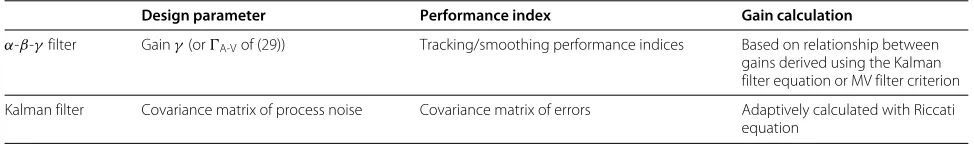
Here, we discuss the design of the α-β-γ filter and compare it with the Kalman filter design. Table 1 sum-marizes the design parameters, performance indices, and gain calculation method for these filters [7,31,32]. (Note that details of the gain design methods of theα-β-γ fil-ter are explained in the next subsection.) As shown in (7) and (8), the above indices can be directly calculated using the filter gains that we have designed. In contrast, for the Kalman filter, we must design the covariance matrix of the process noise. However, the relationship between this and the performance index (error covariance matrix) has not been rigorously established [7,32]. Moreover, the error covariance matrix gives a misleading evaluation of track-ing filter performance, as mentioned earlier in this subsec-tion. Therefore, the design of appropriate process noise is conducted empirically and/or by Monte Carlo simulations (see Section 6 of [6]). Consequently, it is simpler to design an appropriate α-β-γ filter than to construct a Kalman filter or EKF [7,23,26-28].
Gain design methods
Various approaches can be used to determine appropri-ate gains for the α-β-γ filter. The main approach is to derive gains from the Kalman filter equations, because the
α-β-γ filter can be considered as the steady-state Kalman filter [15-17]. However, it is difficult to select appropriate process noise for the motion model, for the same reason as the difficulties in designing a Kalman filter mentioned
in the previous subsection. In addition, the performance of an α-β-γ filter derived from the Kalman filter is not optimal when evaluated using the performance indices expressed in (7) and (8) [31].
To avoid these problems, the MV filter criterion has been proposed [14,31]. This criterion determines the gains by minimizing the smoothing performance indexσp2 under the condition that the tracking performance index efin is constant [31]. As shown in (8), the tracking per-formance index depends only onγ. Thus, for the general
α-β-γ filter, the optimal gains with the MV filter criterion are determined by:
arg min
α,β σ
2 p
sub. to γ =const. (9)
As shown in this equation, the MV filter criterion does not require the process noise of the motion model, unlike the Kalman filter-based approach [15-17]. In [14], it was reported that the performance (evaluated using the tracking/smoothing performance indices of (7) and (8)) is better than that of other α-β-γ filters derived from the Kalman filter equations. Thus, this paper uses the MV filter criterion to determine the optimal gains.
PVMα-β-γfilters
As described in the ‘Introduction’ section, the perfor-mance of PVM tracking filters has not been fully inves-tigated. Hence, we focus on PVMα-β-γ filters. In this section, we derive the smoothing and tracking perfor-mance indices (σp2 and efin) for PVM α-β-γ filters. As mentioned above, we ensure a fair comparison with the generalα-β-γ filter by fixing the number of gains to three. We can define two types of PVMα-β-γ filter. The first has been used in several tracking systems that measure both position and velocity [29,30]. However, its performance indices have not been derived, and thus the gain determi-nation has so far been conducted empirically. The second type is a new PVMα-β-γ filter that is being proposed for the first time in this paper. The aim of this new filter is to achieve accurate tracking, even when the noise in the velocity measurements is comparatively large. The perfor-mance indicesσp2andefinare derived analytically for each PVMα-β-γ filter.
Table 1 Summary of the design and gain calculation of theα-β-γand Kalman filters
Design parameter Performance index Gain calculation
α-β-γfilter Gainγ(orA-Vof (29)) Tracking/smoothing performance indices Based on relationship between gains derived using the Kalman filter equation or MV filter criterion
Acceleration smoothed by measured velocity (A-V)-type PVMα-β-γfilter
Using the measured velocityvok, several researchers have used a PVM α-β-γ filter with the smoothing process [29,30]:
xsk = xpk+α(xok−xpk), (10) vsk = vpk+β(vok−vpk), (11) ask = apk+(γ /T)(vok−vpk), (12)
and a prediction process that is the same as that in the generalα-β-γ filter (expressed in (1) to (3)). Compared with the general α-β-γ filter, the second terms of (5) and (6) have been changed to use the measured veloc-ity. Equation (11) shows that the smoothed velocity can be estimated using the measured velocity. This is the natural expansion of the general α-β-γ filter consider-ing the velocity measurements. Additionally, as shown in (12), the smoothed acceleration is also estimated using the measured velocity. We call this PVMα-β-γ filter the acceleration smoothed by measured velocity (A-V) filter.
The performance indices of the A-V filter are derived from (1) to (3) and (10) to (12). For simplicity, we assume that the noise in the position and velocity measurements is uncorrelated. The smoothing performance index is then derived as
σ2 p, A-V=
α
2−αBx+
f1(α,β,γ ) f2(α,β,γ )
T2Bv, (13)
whereBvis the variance of the noise invok, and
f1(α,β,γ )=α2(β−1)4β2−2βγ−γ2+4γ
+α6β2γ−4β3+8β2+3βγ2−16βγ−2γ21+8γ
−4β2γ +2βγ (4−γ ),
(14)
f2(α,β,γ )=2αβ(2−α)(4−2β−γ )
×α2+αβ+γ −α2β−αβ. (15)
The derivation of (13) is given in the Appendix. Then, the tracking performance index can be derived as
efin, A-V=
12−6β−γ 12αγ JT
3. (16)
Again, details of the derivation are given in the Appendix.
Acceleration smoothed by measured position (A-P)-type PVMα-β-γfilter
As it uses the measured velocity, we expect the A-V fil-ter to realize betfil-ter tracking accuracy than the general
α-β-γ filter. However, the performance of the A-V fil-ter defil-teriorates when the varianceBv is large. To reduce
this deterioration, we consider another PVMα-β-γ filter whose smoothing process is expressed as follows:
xsk = xpk+α(xok−xpk), (17) vsk = vpk+β(vok−vpk), (18)
ask = apk+
γ /T2(xok−xpk), (19) and whose prediction process is the same as in the gen-eralα-β-γ filter (i.e., (1) to (3)). The difference from the A-V filter is that the smoothed acceleration is estimated using the measured position, i.e., (6) in the generalα-β-γ filter. We call this new PVMα-β-γ filter the acceleration smoothed by measured position (A-P) filter. It appears that the performance of the A-P filter is better than that of the A-V filter when Bv is relatively large. In contrast, the A-V filter appears to outperform the A-P filter when Bvis relatively small. Moreover, whenBvis relatively large, it is unclear whether the performance of the A-P filter or the general α-β-γ filter is better. In the next section, these cases are investigated and clarified with theoretical analyses.
We can derive the smoothing performance index for the A-P filter as:
σ2 p, A-P=
g1(α,β,γ )Bx+g2(α,β)T2Bv g3(α,β,γ )
, (20)
where
g1(α,β,γ )=8α3β(2−β)(β−1)
+2α2β3γ+4β3−3β2γ −8β2+6βγ−4γ +αγ2β3+β2γ +4β2−βγ −24β+16 −4βγ (2−β)2,
(21)
g2(α,β)=8β2(α+β−αβ−2), (22)
g3(α,β,γ )=(16−8β−βγ−8α+4αβ)
·2α2β2−2α2β−2αβ2+αβγ−αγ −2βγ+2γ,
(23)
and the tracking performance index is
efin, A-P=JT3/γ. (24)
Note that the tracking performance index is the same as in the generalα-β-γ filter, as shown in (8). The derivation of these performance indices is given in the Appendix.
Performance analysis and comparison
between measurement noise (BxandBv) and filter perfor-mance is clarified for various gain settings.
Optimal gain calculation with MV filter criterion
First, we calculate the optimal gains of the A-V filter. Under the MV filter criterion, we assume that the track-ing performance index is constant. With (16), the tracktrack-ing performance index depends on
CA-V =
12−6β−γ
12αγ . (25)
Thus,CA-Vis constant in the MV filter criterion. Solving this forγ, we obtain
γ = 6(2−β)
12αCA-V+1
. (26)
Substituting (26) into (13) gives the smoothing perfor-mance indexσp, A-V2 (α,β,CA-V), which is used to calculate the optimal gains for constantCA-V. Then, we determine the optimalαandβfor eachCA-Vby:
arg min
α,β σ 2
p, A-V(α,β,CA-V)
sub. to CA-V =const. (27)
Next, we consider the optimal gain calculation of the A-P filter. As shown in (24), the tracking performance index of the A-P filter depends only onγ. Consequently,γ is constant whenefin, A-Pis constant. Thus, we determine the optimalαandβfor eachγ by:
arg min
α,β σ 2 p, A-P
sub. to γ =const. (28)
We now give the gain calculation results using (27) and (28) and compare these with the gains from the GMV filter. First, to simplify the discussion, we define the fol-lowing two parameters.
• The reciprocal ofCA-Vis defined as
A-V=1/CA-V. (29)
With (8), (16), and (24),A-Vcorresponds toγ in the A-P and GMV filters.
• The ratio of the two variances of measurement noise is defined as
Rv=T2Bv/Bx. (30)
The smoothing performance of the PVMα-β-γ filters depends on this ratio, as we can see from (13) and (20). The relationship betweenRvand the performance indices is very important for the design of tracking filters that use both the measured position and velocity.
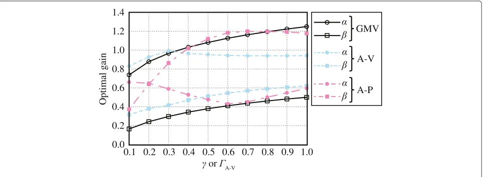
Figure 1 shows the gain calculations for the PVM and GMV filters withRv = 1/2 for each value ofγ orA-V. Here, we have used the gradient descent technique to min-imize (27) and (28); the complexity (using bigOnotation) of this operation isO(n2)[33]. The mean calculation time to determine each(α,β,γ )is 56.3 s using an Intel CORE i7-4600U [email protected] GHz 2.70 GHz. This time is accept-able, because the gain calculation is conducted in the filter design process before its application in a tracking system. As shown in Figure 1, the value ofβin the A-V filter is rel-atively large compared with that in the GMV filter. This is becauseβis the gain for velocity smoothing, and the mea-surement accuracy of the velocity is better than that of the position. For the same reason, the value ofβ(α) is larger (smaller) in the A-P filter than in the other filters. These examples indicate that the gains of the PVM filters depend on the relationship between the accuracy of the position and velocity measurements.
0.0 0.2 0.4 0.6 0.8 1.0 1.2 1.4
0.1 0.2 0.3 0.4 0.5 0.6 0.7 0.8 0.9 1.0
or A-V
Optimal gain
GMV
A-V
A-P
Analysis results and discussion
Using the calculated optimal gains, we conduct perfor-mance analyses of the A-V, A-P, and GMV filters. The smoothing performance indices of these filters are calcu-lated using (7), (13), and (20) under the assumption that the tracking performance indices are constant (i.e.,A-Vis constant for the A-V filter andγ is constant for the other filters). We assume that the sampling intervalT and the variance of the measured position errorBxare normalized to 1.
Figure 2 shows the smoothing performance indices as a function of γ or A-V forRv = 1/2 and 7. For rel-atively small Rv, shown in Figure 2a, the PVM α-β-γ filters outperform the GMV filter, especially for large val-ues ofγ orA-V. In this case, the A-V filter realizes the best performance. This is because accurately measured velocities improve the performance of both the smooth-ing and tracksmooth-ing. Moreover, for larger values ofRv, shown in Figure 2b, the performance deterioration in the pro-posed A-P filter is small compared with that in the A-V filter. This is because the smoothed acceleration in the A-P filter is calculated using the measured position. The smoothing performance of the A-P filter is better than that of the GMV filter when γ ≥ 0.6 forRv = 7. This result implies that the proposed A-P filter can realize bet-ter performance than the GMV filbet-ter, even when the noise in the velocity measurements is large. Figure 3 shows the smoothing performance indices as a function ofRvforγ andA-Vvalues of 0.9. As shown in this figure, forRv=10 (i.e., the noise variance in the velocity measurements is ten times as large as that in the position measurements), the
0
1
2
3
4
5
6
7
8
9
0.1
1
10
Smoothing performance index
R
VGMV
A-V
A-P
Figure 3Relationship between smoothing performance indices and the ratioRvwhenA−V=γ=0.9.
A-P filter achieves better smoothing performance than the GMV filter. In contrast, the performance of the A-V filter deteriorates whenRvis comparatively large.
Table 2 summarizes the properties of theα-β-γ filters considered in this paper. This table indicates that the A-V filter realizes accurate tracking for smallRv, whereas the proposed A-P filter realizes better accuracy than the other filters for relatively large Rv. Additionally, when
0
1
2
3
4
5
6
7
8
0.1 0.2 0.3 0.4 0.5 0.6 0.7 0.8 0.9 1.0
GMV
A-V
A-P
0
1
2
3
4
5
6
7
8
0.1 0.2 0.3 0.4 0.5 0.6 0.7 0.8 0.9 1.0
GMV
A-V
A-P
or
A-Vor
A-VSmoothing performance index
Smoothing performance index
(a)
(b)
Table 2 Summary of the properties of theα-β-γfilters considered in this paper
GMV filter A-V filter A-P filtera
Measurement parameter Position Position and velocity
Prediction process (1) to (3)
Smoothing process (4) to (6) (10) to (12) (17) to (19)a Smoothing performance index (7) (13)a (20)a Tracking performance index (8) (16)a (8)a Suitable whenRvis very largea smalla largea aIndicates novel results in this paper.
Rv becomes large, the GMV filter realizes the best per-formance, which suggests that we should not use the measured velocity in this case.
Cramér–Rao bound evaluation
This section calculates the fundamental performance lim-itation of the PVM and conventional tracking problems using a Cramér–Rao bound (CRB) evaluation. Moreover, we evaluate the tracking accuracy of the PVM filters using Monte Carlo simulations and compare this with the CRBs. The CRBs in the position estimation are calculated by the Riccati-like recursion used in [34]. The CRB is the lower bound of the covariance of the state estimation, which is expressed as
Exˆk−xtk xˆk−xtk T≥
J−k1=Pk, (31)
wherexˆkis the target state estimate based on all measure-ments collected up to and including time kT, the target state is composed of the position, velocity, and accelera-tion in the form(xk,vk,ak)T,Jkis the filtering information
matrix defined in [35], andPk is the CRB. When we do not use the process noise, the recursive formula forJkcan be expressed as [36]:
Jk+1=
F−1TJkF−1+HTR−1H, (32) whereFis the state transition matrix,His the observation matrix, and R is the covariance matrix of measurement noise. In the PVM tracking problem, these are expressed as [26]:
F =
⎛
⎝1 T T
2/2
0 1 T
0 0 1
⎞
⎠, (33)
H =
1 0 0 0 1 0
, (34)
R=
Bx 0
0 Bv
. (35)
A detailed explanation is provided in [34].
First, we calculate and compare the CRBs of the gen-eral position-only-measured and PVM tracking problems. In the position-only-measured tracking problem,HandR
are expressed as:
H =1 0 0, (36)
R=Bx
, (37)
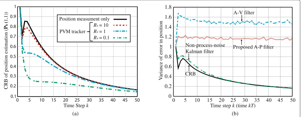
andFis same as (33). We setBx=1 andT =1. Figure 4a shows the calculated CRBs of the position estimation. As shown in this figure, the performance limitation of the PVM tracking problem is less than that of the position-only-measured tracking problem. The limitation of the PVM tracking problem withRv=0.1 is small even for rel-atively largek. WhenRv=10, the CRB is almost the same as that for the position-only-measured tracking problem
(a) (b)
Time step k (time kT)
V
ariance of error in position
Time Step k
CRB of position estimation (
P
k
(
1,1))
Rv = 10 Rv = 1 Rv = 0.1 Position measument only
PVM tracker
A-V filter
Proposed A-P filter
CRB
0 1
0.2 0.4 0.6 0.8 1.2 1.4 1.6 1.8
Non-process-noise Kalman filter
at approximatelyk>10. However, no deterioration in the CRBs has occurred.
Next, we compare the CRBs with the performance of the PVMα-β-γ filters calculated using Monte Carlo sim-ulations. We set the number of Monte Carlo simulations to 10,000, the initial state to (0, 0.5, 0.005)T, Bx = 1, andT = 1. For reference, the simulation results for the non-process-noise Kalman filter [32] are also presented. Figure 4b shows the CRB and the Monte Carlo simula-tion results for the A-V and A-P filters forγ (A-V)=0.1 and the non-process-noise Kalman filters whereRv =10. As shown in this figure, the accuracy of the PVM α
-β-γ filters is worse than that of the non-process-noise Kalman filter whose performance is close to the CRB. This is because the α-β-γ filter uses fixed gains, unlike the Kalman filter. However, the proposed A-P filter produces a smaller difference between the CRBs and error variances than the A-V filter. Additionally, the computational load of the proposed filter is smaller than that of the Kalman filter, as we shall discuss later.
Simulation assuming radar tracking of a maneuvering target
Finally, we use numerical simulations to investigate the performance of each filter for a realistic maneuvering tar-get. In this subsection, we simulate the Doppler radar tracking [20,21,29] of a maneuvering target and compare the tracking errors given by the three filters considered in this paper and an EKF [1,2]. Figure 5 shows the simulation scenario. Figure 5a,b shows the true target motion and the radar position, respectively. Two-dimensional (2D) track-ing of the point target is assumed, and the received radar signals are calculated using ray-tracing, as in [29]. We
assume there are two Doppler radars located at(x,y) = (0, 0) and (0.5 m, 0). The sampling interval T is 1 ms, and the transmitting signal is an ultrawide-band pulse with a center frequency of 26.4 GHz and bandwidth of 2 GHz. The radars measure the position using ranging results and the velocity using the Doppler shift [29]. White Gaussian noise is added to the ranging and Doppler shift estimations to controlRv. Figure 5c shows the true target position at each time.
We now describe the composition of the tracking filters. For 2D tracking, theα-β-γ filter is composed as follows tion, velocity, and acceleration along the x-axis, yk, vyk, andayk denote position, velocity, and acceleration along they-axis, and subscripts ‘s’, ‘p’, and ‘o’ denote ‘smoothed’, ‘predicted’, and ‘observed (measured)’, respectively. In the
0.65
A-V filter tracking,Kis expressed as:
In the A-P filter tracking,Kis expressed as:
KA-P=
Additionally, in the EKF tracking,K is the Kalman gain matrix calculated by the Kalman filter equations, and a
nonlinear measurement model is used [1]. The EKF con-siders the correlation between thex−yaxes, unlike the
α-β-γ filters. The process noise is taken to be the zero-mean random-acceleration noise given in [2], and we empirically set this to realize errors that are as small as possible.
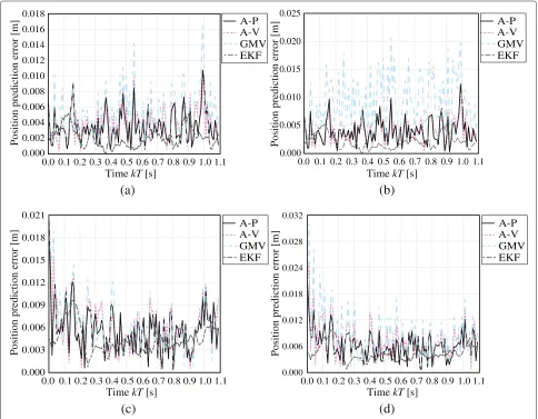
Figure 6 shows the results of the 2D radar track-ing. Figure 6a,b shows the position prediction error
(xpk−xtk)2+(ypk−ytk)2(whereytkis the truey) forγ andA-V values of 0.2 and 0.8 with the GMV and PVM α-β-γ filters when the meanRvis 0.426. The gains of the GMV and PVMα-β-γ filters are calculated according to this mean Rv. As for the previous analyses and simula-tions, the accuracy of the PVMα-β-γ filters is somewhat better than that of the GMV filters when the gains are relatively large. In both cases, the EKF realizes the best performance. This is because it considers the correlated noise of the axes and has four times as many gains as
0.000
Position prediction error [m] Position prediction error [m]
Position prediction error [m] Position prediction error [m]
theα-β-γfilters. Moreover, these gains change adaptively. However, the PVM α-β-γ filters realize relatively good accuracy with fixed gains and a small computational load. Table 3 shows the required number of addition, multipli-cation, and inversion operations of matrices for each time stepkfor the EKF and PVMα-β-γ filter. As shown in this table, the computational load of the PVMα-β-γ filter is smaller than that of the EKF.
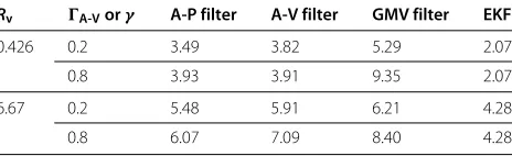
Next, we present results for when the velocity surement noise is large compared with the position mea-surement noise. Figure 6c,d shows the position prediction error forγ andA-V values of 0.2 and 0.8 with the GMV and PVM α-β-γ filters when the mean Rv is 6.67. The EKF realizes the best performance in both cases, as for the previous scenario. Whenγ = A-V = 0.2, the differ-ence between the threeα-β-γ filters is slight, as suggested by our theoretical analysis. Whenγ = A-V = 0.8, the proposed A-P filter realizes slightly better accuracy than the other twoα-β-γ filters. Table 4 lists the mean error of the results shown in Figure 6. From this table, we can see that the mean accuracy of the EKF is better than that of the PVMα-β-γ filters in all cases. However, the accuracy of the PVMα-β-γ filters is sufficiently high. As shown in Figure 6, the positioning errors of the PVMα-β-γ filters are almost smaller than the wavelength of the radar signal (which is approximately 0.0114 m, corresponding to 26.4 GHz). For various remote sensing applications using radar, sonar, and laser, an accuracy of better than the wavelength is often expected. Thus, the above results indicate that the accuracy of the PVM filters is sufficient for various remote sensing applications. In contrast, the errors in the GMV filter are often larger than the wavelength. The mean error of the A-V filter is 0.418 times that of the GMV filter when Rv = 0.426 andγ = A-V = 0.8. Moreover, the A-P filter even realizes better accuracy whenRv = 6.67. These results indicate that the PVM filters enable accurate tracking with simple calculations and few gains when the velocity measurement noise is relatively small, even for 2D radar tracking applications.
Conclusions
In this paper, we have examined the performance of two PVMα-β-γ filters: the A-V filter and the newly proposed A-P filter. The A-V filter estimates smoothed acceleration using the measured velocity, whereas the proposed A-P filter uses the measured position. We analytically derived the tracking and smoothing performance indices of each
Table 3 Required number of matrix operations for the tracking filtering in each time step
Addition Multiplication Inversion
PVMα-β-γfilter 1 2 0
EKF 5 11 1
Table 4 Mean of the predicted errors in 2D radar simulations (units: mm)
Rv A-Vorγ A-P filter A-V filter GMV filter EKF
0.426 0.2 3.49 3.82 5.29 2.07
0.8 3.93 3.91 9.35 2.07
6.67 0.2 5.48 5.91 6.21 4.28
0.8 6.07 7.09 8.40 4.28
filter. Based on these performance indices, we calculated the optimal gains of the PVMα-β-γ filters with the MV filter criterion. The performance of the A-V and A-P fil-ters was investigated in terms of the calculated gains, and we compared the output with that from the GMV filter. Numerical analyses verified that the A-V filter real-izes better accuracy than the GMV filter when the ratio Rv is relatively small. Moreover, the proposed A-P fil-ter achieved betfil-ter performance when both Rv and the gainγ were comparatively large. The proposed A-P filter achieved the best performance forRv=7 andγ ≥0.6. In particular, even forRv = 10, which means that the vari-ance of noise in the velocity measurements is ten times that in the position measurements, the A-P filter was more accurate than the GMV filter when γ = 0.9. Finally, numerical simulations verified the effectiveness of the A-V and A-P filters for a realistic 2D radar application. More-over, the simulation results matched those from numerical analyses using the derived performance indices. Thus, the performance analyses presented in this paper will be use-ful for the design of actual tracking systems using position and velocity measurements. One limitation of the current study is our assumption that there are three filter gains. The relaxation of this assumption is an important area of future work that will enable the realization of more accurate tracking filters.
Appendix Derivation of (13)
The true position of a target under constant acceleration is expressed as
xtk =xtk−1+Tvtk−1+
T2/2atk−1, (42) where vt and at are the true velocity and acceleration. With (1) and (42), the variance of the predicted position errors is
σ2 p =E
xpk−xtk
2
=Exsk−1−xtk−1 2
+T2Evsk−1−vtk−1 2
+T4/4Eask−1−atk−1 2
+2TExsk−1−xtk−1 vsk−1−vtk−1
+T2Exsk−1−xtk−1 ask−1−atk−1
+T3Evsk−1−vtk−1 ask−1−atk−1.
Because we assume a steady state, the variances and covariances in (43) do not depend onk. Consequently, we can define these variances and covariances as:
σ2
Substituting (44) to (49) into (43), we have
σ2
p=σsx2 +T2σsv2 +
T4/4σsa2 +2Tσsxv2 +T2σsxa2 +T3σsva2 .
(50)
The variances and covariances in this equation are derived as functions of the filter gains and the variances of mea-surement noise. With (1) and (10), we have
xsk=(1−α)
We can rewrite (42) as
xtk =(1−α)
Using (51) and (52), the smoothing error is expressed as xsk−xtk = (1−α) Thus, the variance of this error is calculated as
σ2
The following relations are satisfied because of the steady-state assumption and because the smoothed parameters are a linear combination of the measured parameters:
Exsk−1−xtk−1 Substituting (44) to (49) and (55) to (58) into (54), we obtain This can be simplified to
α(2−α)σsx2 −(1−α)2T2σsv2+T4/4σsa2 +2Tσsxv2
+T2σsxa2 +T3σsva2 =α2Bx. (60) In the same way, other variances and covariances are calculated using (1) to (3) and (10) to (12) as follows:
σ2
and the following is satisfied because we assume that the measurement position and velocity noise are uncorrelated:
Equations (61) to (65) can be simplified to:
Solving the linear system involving (59) and (68) to (72), we obtain: (15). Substituting (73) to (78) into (50), we arrive at (13).
Derivation of (16)
We first derive the relationship between the measured sig-nals (xok andvok) and the predicted positionxpk in the z-domain and then obtain the tracking performance index using the final value theorem. Applying az-transform to (1) to (3) and (10) to (12), we obtain:
Substituting (84) into (81), we have
Ap(z) = γ z−1 ·
Vo(z)−Vp(z)
T . (85)
Substituting (83) into (80) gives
(z+β−1)Vp(z) = βVo(z)+zTAp(z). (86)
Substituting (85) into (86), the relationship between the predicted and measured velocities is calculated as
Vp(z) = (β+γ ) z−β
z2+(β+γ −2)z−β+1Vo(z). (87)
Substituting (87) into (85), the relationship between the predicted acceleration and the measured velocities is cal-culated as
Substituting (82) to (84), (87), and (88) into (79), the rela-tionship between the predicted position and the measured position and velocity is written as
Xp(z)= α
Here, the measured position and velocity of a target with constant jerkJare:
xok = J(kT)3/6, (91)
vok = J(kT)2/2, (92)
and theirz-transforms are:
Xo(z) =
Substituting (93) and (94) into (90), we have
Derivation of (20)
Using the same procedure as for the A-V filter, the linear system with respect to the variances and covariances of the smoothing parameters is calculated using (1) to (3) and (17) to (19) as:
α(2−α)σsx2 −(1−α)2T2σsv2+T4/4σsa2 +2Tσsxv2
+T2σsxa2 +T3σsva2 =α2Bx,
(96)
β(2−β)σsv2 −(1−β)2T2σsa2+2Tσsva2 =β2Bv, (97)
(γ (4−γ )/4) σsa2 −γ −2/T4 σsx2 +T2σsv2 +2Tσsxv2
+γ (2−γ )σsxa2 /T2+σsva2 /T=γ2/T4Bx,
(98)
(α+β−αβ) σ2
sxv−(1−α)(1−β)
Tσsv2+T3/2σsa2 +Tσsxa2 +(3T2/2)σsva2 σsxv2 =0, (99)
(α+γ−αγ ) σ2
sxa−(α−1)(γ −1)Tσsva2
−((α−1)(γ −2)/4)T2σsa2
+γ (1−α)(σsx2/T2+σsv2 +2σsxv2 /T)=αγ /T2Bx, (100)
(2β+3γ −3βγ ) σsva2 /2+γ (1−β) ×σ2
sxv/T2+σsv2/T+σsxa2 /T2
−(β−1)(γ −2)Tσsa2/2=0.
(101)
Solving the linear system involving (96) to (101), we obtain:
σ2 sx=
g1x(α,β,γ )Bx+(1−α)2g2(α,β)T2Bv g3(α,β,γ )
, (102)
σ2 sv=
g1v(α,β,γ )Bx/T2+g2v(α,β,γ )Bv (2−β)g3(α,β,γ )
, (103)
σ2 sa=
g1a(α,β,γ )Bx/T4+g2a(α,β,γ )Bv/T2 (2−β)g3(α,β,γ )
, (104)
σ2 sxv=
g1xv(α,β,γ )Bx/T+g2xv(α,β,γ )TBv g3(α,β,γ )
, (105)
σ2
sxa=
g1xa(α,β,γ )Bx/T2+2(1−α)(2−β)γ2g2(α,β)Bv
γ (2−β)g3(α,β,γ )
,
(106)
σ2 sva=
g1va(α,β,γ )Bx/T3+g2va(α,β,γ )Bv/T (2−β)g3(α,β,γ )
,
(107)
whereg2(α,β)andg3(α,β,γ )are expressed as (22) and (23), and
g1x(α,β,γ )=8α3β(2−β)(β−1)−2α23β3γ −4β3
−9β2γ +8β2+2βγ+4γ
+αγ10β3+β2γ−28β2−βγ +8β+16 −4βγ (2−β)2,
(108)
g1v(α,β,γ )= 8γ2(1−β)2(2−β)(α+β−αβ−2), (109)
g2v(α,β,γ )=8α3β2(2−β)(1−β)+2α2β2(β−2)
×(3βγ−12β−3γ +8)
−αβ222β2γ −16β2+βγ2−64βγ
+32β−γ2+40γ
+2β2γ (β−1)(8β+γ −16),
(110)
g1a(α,β,γ )=4βγ2(β−2)
2αβ2−6αβ−2β2−βγ +4α+4β+γ ),
(111)
g2a(α,β,γ )=4β2γ (α−2)2αβ2−6αβ−2β2−βγ
+4α+4β+γ ),
(112)
g1xv(α,β,γ )=2βγ (α−1)(β−2)(β−1)(4α+γ ), (113)
g2xv(α,β,γ )=2β2(α−1)(α−2)(β−1)(4α+γ ), (114)
g1xa(α,β,γ )=γ2(2−β)
8α2β3−24α2β2+16α2β +2αβ3γ −8αβ3−6αβ2γ +16αβ2 −4αβγ +8αγ −2β3γ −β2γ2+βγ2 +16βγ−16γ,
(115)
g1va(α,β,γ )=2βγ2(2−β)(β−1)(4αβ−8α−4β−γ+8),
(116)
g2va(α,β,γ )=2β2γ (2−α)(β−1)(4αβ−8α−4β−γ+8).
(117)
Substituting (102) to (107) into (50), we arrive at (20).
Derivation of (24)
and their simplified forms, the predicted parameters in the z-domain are derived as:
Ap(z)= γ
Substituting (118) and (119) into (120), the relationship between the predicted position and the measured position and velocity is expressed as
Xp(z)=
From (121), thez-transform of the predicted error is
Ep(z)=Xo(z)−Xp(z)
Substituting (93) and (94) into (124), the error for a target with constant jerk is given by
Ep(z) =
zz2−2βz+4z−β+1 3(z−1)h2(z)
JT3. (125)
Applying the final value theorem to (125), we have (24).
Abbreviations
PVM: position-velocity-measured; MV: minimum-variance; A-V filter: acceleration smoothed by measured velocity-type PVMα-β-γfilter; A-P filter: acceleration smoothed by measured position-type PVMα-β-γfilter; GMV filter: general minimum-varianceα-β-γfilter; CRB: Cramér–Rao bound; EKF: extended Kalman filter.
Competing interests
The authors declare that they have no competing interests.
Acknowledgements
This work was supported in part by the Ministry of Internal Affairs and Communications of Japan and JSPS KAKENHI Grant Number 26880023.
Received: 15 September 2014 Accepted: 18 March 2015
References
1. MJ Jahromi, HK Bizaki, Target tracking in MIMO radar systems using velocity vector. J. Inf. Sys. Telecommun.2, 150–158 (2014)
2. K Dae-Bong, H Sun-Mog, Multiple-target tracking and track management for an FMCW radar network. EURASIP J. Adv. Sig. Proc.2013, 159 (2013) 3. H Cheng, Z Tao, Z Chao, Accurate three-dimensional tracking method in
bistatic forward scatter radar. EURASIP J. Adv. Sig. Proc.2013, 66 (2013) 4. H Niknejad, A Takeuchi, S Mita, D McAllester, On-road multivehicle
tracking using deformable object model and particle filter with improved likelihood estimation. IEEE Trans. Intel. Transport. Sys.13, 748–758 (2012) 5. M Daun, F Ehlers, Tracking algorithms for multistatic sonar systems.
EURASIP J. Adv. Sig. Proc.2010, 461538 (2010)
6. B Ekstrand, Some aspects on filter design for target tracking. J. Control Sci. Eng., 870890 (2012)
7. Y Bar-Shalom, XR Li, T Kirubarajan,Estimation with Applications to Tracking and Navigation. (Wiley-Interscience, New York City, USA, 2001) 8. D Tenne, T Singh, Characterizing performance ofα-β-γfilters. IEEE Trans.
Aero. Elec. Sys.38, 1072–1087 (2002)
9. NH Khin, YF Che, SML Eileen, WX Liang, Alpha beta gamma filter for cascaded PID motor position control. Procedia Eng.41, 244–250 (2012) 10. YS Lee, HJ Lee, inProc. of Int. Conf. Advanced Communication Technology
2009 (ICACT2009). Multiple object tracking for fall detection in real-time surveillance system (IEEE Phoenix Park, 2009), pp. 2308–2312 11. Y Wang, Feature point correspondence between consecutive frames
based on genetic algorithm. Int. J. Robot. Automation.21, 35–38 (2006) 12. K Daniilidis, C Krauss, M Hansen, G Sommer, Real-time tracking of moving
objects with an active camera. Real-Time Imaging.4, 3–20 (1998) 13. Y Kosuge, M Ito, T Okada, S Mano, Steady-state errors of anα-β-γfilter for
radar tracking. Electron. Commun. Japan (Part III: Fundamental Electronic Sci.)85, 65–79 (2002)
14. Y Kosuge, M Ito, inProc. of the 40th SICE Annual Conf. A necessary and sufficient condition for the stability of anα-β-γfilter (The Society of Instrument and Control Engineers Nagoya, 2001), pp. 7–12
15. CC Arcasoy, G Ouyang, Analytical solution ofα-β-γtracking filter with a noisy jerk as correlated target maneuver model. IEEE Trans. Aero. Elec. Sys. 33, 347–353 (1997)
16. JJ Sudano, Theα-β-γtracking filter with a noisy jerk as the maneuver model. IEEE Trans. Aero. Elec. Sys.29, 578–580 (1993)
17. PR Kalata, The tracking index: A generalized parameter forα-βandα-β-γ target trackers. IEEE Trans. Aero. Elec. Sys.AES-20, 174–182 (1984) 18. W Chun-Mu, C Ching-Kao, C Tung-Te, A new EP-basedα-β-γ-δfilter for
target tracking. Math. Comput. Simul.81, 1785–1794 (2011) 19. D Mohammed, K Mokhtar, O Abdelaziz, M Abdelkrim, A new IMM
algorithm using fixed coefficients filters (fastIMM). Int. J. of Electron. Commun. (AEÜ).64, 1123–1127 (2009)
20. R Kozma, L Wang, K Iftekharuddin, E McCracken, M Khan, K Islam, SR Bhurtel, RM Demirer, A radar-enabled collaborative sensor network integrating COTS technology for surveillance and tracking. Sensors.12, 1336–1351 (2012)
21. JH Lim, A Terzis, I-J Wang, inProc. of 2010 IEEE 35th Conf. Local Computer Networks (LCN). Tracking a non-cooperative mobile target using low-power pulsed Doppler radars (IEEE Denver, CO, 2010), pp. 913–920 22. YJ Hong, KD Yong, BS Hwan, S vladimir, Joint initialization and tracking of
multiple moving objects using Doppler information. IEEE Trans. Sig. Proc. 59, 3447–3452 (2011)
23. BR Geetha, KV Ramachandra, A three state Kalman filter with range and range-rate measurements. Int. J. Comput. Appl.3, 85–101 (2013) 24. X Zhu, J Hong, W Cui, inProc. of 4th IEEE Conf. on Industrial Electronics and
Applications 2009. Study on radar data processing algorithm with improved Kalman filter (IEEE Xi’an, 2009), pp. 3826–3829
25. K Jonghyuk, S Salah, 6DoF SLAM aided GNSS/INS navigation in GNSS denied and unknown environments. J. Global Pos. Sys.4, 120–128 (2005) 26. KV Ramachandra, BR Mohan, BR Geetha, A three-state Kalman tracker
using position and rate measurements. IEEE Trans. Aero. Elec. Sys.29, 215–222 (1993)
28. FR Castella, Tracking accuracies with position and rate measurements. IEEE Trans. Aero. Elec. Sys.AES-17, 433–437 (1980)
29. H Yamazaki, K Saho, T Sato, inProc. of 10th International Conference on Space, Aeronautical and Navigational Electronics. Accurate shape estimation method for multiple moving targets with UWB Doppler radar interferometers (IEICE Hanoi, 2013), pp. 7–12
30. C Zheng,Tracking vehicular motion-position using V2V communication. (Master’s thesis, the University of Waterloo, 2010)
31. Y Kosuge, M Ito, Evaluating anα-βfilter in terms of increasing a track update-sampling rate and improving measurement accuracy. Electron. Commun. in Japan (Part I: Communications).86, 10–20 (2003) 32. Y Kosuge, inProc. of SICE Annual Conference, 2008. Non-process-noise
tracking filter using a constant velocity model (The Society of Instrument and Control Engineers Tokyo, 2008), pp. 2670–2674
33. P Baldi, Gradient descent learning algorithm overview: A general dynamical systems perspective. IEEE Trans. Neural Netw.6, 182–195 (1995) 34. B Ristic, A Farina, M Hernandez, Cramér-Rao lower bound for tracking
multiple targets. IEE Proc. Radar Sonar Navig.151, 129–134 (2004) 35. P Tichavsky, CH Muravchik, A Nehorai, Posterior Cramér-Rao bounds for
discrete-time nonlinear filtering. IEEE Trans. Sig. Process.46, 1386–1396 (1998)
36. B Ristic, A Farina, D Benvenuti, MS Arulampalam, Performance bounds and comparison of nonlinear filters for tracking a ballistic object on reentry. IEE Proc. Radar Sonar Navig.150, 65–70 (2003)
Submit your manuscript to a
journal and benefi t from:
7Convenient online submission
7Rigorous peer review
7Immediate publication on acceptance
7Open access: articles freely available online
7High visibility within the fi eld
7Retaining the copyright to your article