A Robust Sub-Integer Range Alignment Algorithm Against MTRC for ISAR Imaging

(1)

A Robust Sub-Integer Range Alignment Algorithm against MTRC

for ISAR Imaging

Pengjiang Hu*, Shiyou Xu, and Zengping Chen

Abstract—Range alignment plays an important role in the inverse synthetic aperture radar (ISAR) imaging. The performance of the traditional range alignment algorithms decreases when the migration through resolution cells (MTRC) is much severe. In this paper, a measure of MTRC is defined, and the effect of MTRC on range alignment is analyzed. Taking MTRC into account, a robust sub-integer range alignment algorithm is proposed. Firstly, each range profile is interpolated to remove the precision limitation of integer range resolution cell. Subsequently, the matrix formed by all the range profiles is partitioned into several matrix blocks on the slow-time domain. For each matrix block, the range profiles are aligned by minimizing the entropy of the average range profile (ARP). Finally, the matrix blocks are coarsely aligned using the maximum correlation method, followed by a fine alignment based on the minimization of the ISAR image entropy. The effectiveness of the proposed algorithm is validated by simulations and real-world data. Results demonstrate that the proposed method is robust against MTRC and can reduce the alignment error. The resultant ISAR image is much better focused.

1. INTRODUCTION

Due to the high-resolution imaging ability of remote moving targets, the inverse synthetic aperture radar (ISAR) imaging has been widely applied in military and civilian applications [1–4], which can help obtain numerous characteristics of the target. For ISAR imaging technology, a wide-band signal is transmitted to achieve high range resolution, while the cross-range resolution is based on an appropriate coherent integration angle.

Range-Doppler (RD) imaging algorithm based on the turntable model is widely used in ISAR realms [5]. However, for a non-cooperative target, the relative radar-target motion usually consists of the translation of an arbitrary reference point and the rotation around that point. While the rotation is the necessary prerequisite to resolve diﬀerent scatterers in the cross-range domain, the translation needs to be compensated accurately before performing the RD algorithm. After that, the target observation can be treated as a turntable model.

As illustrated above, the translation between the target and the radar leads to envelope shift and doppler phase errors. Hence, range alignment and phase adjustment are usually conducted successively according to diﬀerent compensation precision requirements. Based on the adopted criterion, the already existed range alignment algorithms in open articles can be divided into four kinds, namely, cross-correlation [1, 6, 7], entropy minimization [8, 9], contrast maximization [10] and frequency-domain method [1]. In terms of phase adjustment, the prominent scatterer algorithm [11], doppler centroid tracking [12], phase gradient autofocus [13], entropy minimization [14–19] and contrast maximization [18, 20] are regarded as the outstanding representatives.

Received 9 May 2017, Accepted 3 July 2017, Scheduled 17 July 2017

* Corresponding author: Pengjiang Hu ([email protected]).

(2)

In the ISAR imaging process, range alignment is the pre-condition of phase adjustment, and the performance of phase adjustment depends on the range alignment precision. Therefore, a high precision range alignment algorithm is significantly important to the ISAR image quality. The aforementioned range alignment algorithms are inherently based on the similarity of adjacent range profiles. The scatterers are assumed to be located in the same range cell during the coherent processing interval (CPI). These methods are effective when the rotation angle is small and the signal bandwidth is not too wide. However, with the increase of the transmitted signal bandwidth, the scintillation and migration through resolution cells (MTRC) of the scatterers become severe, and the similarity between adjacent range profiles is destroyed. As a result, the performance declines and the resultant ISAR image would be fairly disappointing.

To tackle this problem, we first study the effect of MTRC on range alignment and define a indicator to measure the MTRC. Then we take the MTRC into account and propose a robust three-step sub-integer range alignment method. Concretely, the sub-integer range alignment is based on the interpolation of the range profiles. The robust range alignment against MTRC is based on the matrix partition. Specially, the range profile matrix is partitioned into several matrix blocks through the slow time. For each matrix block, the range profiles are aligned by minimizing the entropy of the average range profile (ARP). Then the ARP of each matrix block are used to align the matrix blocks coarsely using maximum correlation method, a fine alignment is obtained based on the minimization of the ISAR image entropy.

The rest of the paper is organized as follows. In Section 2, the ISAR imaging model is introduced. In Section 3, the eﬀect of MTRC on traditional range alignment algorithms is analyzed, and in Section 4, we present the proposed algorithm. Experimental results and analysis are given in Section 5. Finally, some conclusions are drawn in Section 6.

2. SHORT REVIEW OF THE ISAR IMAGING PROCESS AND THE DERIVATION OF THE SIGNAL MODEL

In this section, the ISAR imaging principle is brieﬂy introduced, and the imaging model is derived. Without loss of generality, we assume that the target moves within the 2-D plane. The ISAR imaging

X

Y

0,m

R

,

k m

R

,

k m k m

P

(

x

y

)

O

,

k m k

r

θ

,

(3)

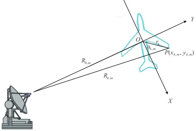
geometry is depicted in Fig. 1. Coordinate system (O, X, Y) has its origin on the reference point of the target, Y-axis is the radar line of sight (RLOS), and X-axis is perpendicular to RLOS. According to the cosine theorem, the distance between thekth scatterer P(xk,m, yk,m) and the radar at slow timetm is given by

Rk,m=

R2

0,m+rk2+ 2R0,mrksin(θk,m) (1)

where R0,m is the range from the reference point to radar, rk =

x2_k,m+y2_k,m the modulus of −−→OP,

and θk,m the angle between −−→OP and the X-axis (measured counter-clockwise from the X-axis). The subscriptm represents the slow time tm =mT, where T is the reciprocal of pulse repetition frequency (PRF). For large distance,R0,mrk, Eq. (1) can be approximated as

Rk,m≈R0,m+rksin(θk,m) (2)

Since the CPI is usually short, the translational motion and rotation are usually modeled as uniform. Thus,R0,m and θk,m can be assumed to change linearly and can be written in the formula

R0,m=R0+V tm

θk,m=θk,0+ωtm

(3)

where R0 and θk,0 denote the initial distance and initial angle, respectively. V and ω are the constant speed of translational motion and rotation, respectively. Substituting Eq. (3) into Eq. (2), we can obtain

Rk,m=R0+V tm+rksin(θk,0) cos(ωtm) +rkcos(θk,0) sin(ωtm) (4) In the case of a small integration angle, cos(ωtm)≈1 and sin(ωtm)≈ωtm, which leads to

Rk,m=R0+V tm+yk,0+xk,0ωtm (5)

Assuming that the radar transmits linear frequency modulated (LFM) signal, the mth echo from the target is processed with dechirp and Fourier transform. After the compensation of the residual video phase (RVP), the range proﬁle of the target can be obtained [21]

sm(fi) =

K

i=1

AkTpsinc

Tp

fi+ 2γ

cRΔk,m

exp

−j4π

c fcRΔk,m

(6)

whereTp, γ, K, Ak are the pulse width, the frequency-modulated rate, the number of scatterers and the backscattered ﬁeld amplitude of thekthscatterer, respectively. fc andfirepresent the carrier frequency and the beat frequency, respectively. RΔk,m =Rk,m−Rref,m denotes the algebraic diﬀerence between

Rk,m and the reference range Rref,m. Let M denote the number of coherent processing pulses and

E={1, . . . , M} denote the slow time sequences. If

Rref,m=R0+V tm, m∈E (7)

Then Eq. (6) can be written as

sm(fi) =

K

i=1

AkTpsinc

Tp

fi+ 2γ

c(yk,0+xk,0ωtm)

exp

−j4π

c fc(yk,0+xk,0ωtm)

(8)

Based on Eq. (8), the ISAR image can be easily constructed by performing Fourier transform with respect to slow time for every range cell.

In real-world applications, however, the reference range deviation ϑm always exists, thus

Rref,m=R0+V tm+ϑm, m∈E (9)

Substituting Eqs. (5) and (9) into Eq. (6), we have

sm(fi) =

K

i=1

AkTpsinc

Tp

fi+ 2γ

c(yk,0+xk,0ωtm−ϑm)

exp

−j4π

c fc(yk,0+xk,0ωtm−ϑm)

(10)

(4)

3. THE EFFECT OF MTRCS ON RANGE ALIGNMENT

Hitherto, the existing translational motion compensation algorithms all assume that the migration of the scatterers is within one resolution cell during the CPI. But it can be seen from Eq. (8) that the termxk,0ωtm may lead to the MTRC. The MTRC can be ignored for low resolution radar but must be accounted for under high resolution condition. We define the ratioωM T /ρr as a measure of MTRC for the same target in different resolutionρr. The ratio is inversely proportional to the range resolutionρr. With the improvement of resolution, the scatterers may migration through several resolution cells, and then MTRC cannot be ignored. Consequently, the similarity is greatly destroyed. The MTRC can be easily eliminated through Keystone transform [21], however, the Keystone transform must be carried out after translational motion compensation. Thus the classical range alignment algorithm performance will be affected by MTRC.

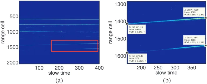
A set of real-world data of some target collected by an experimental radar is utilized to demonstrate the MTRC phenomenon. 400 target returns were recorded and the range profiles are shown in Fig. 2(a). The range profiles in the red box is magnified and shown in Fig. 2(b). Two strong scatterers are observed. As we can see, the scatterer on the top migrates from the 1415th range cell to the 1380th range cell, and the scatterer on the bottom migrates from the 1583th range cell to the 1541th range cell. It is clearly noted that the MTRC is much severe and cannot be ignored.

slow time

range cell

100 200 300 400 500

1000

1500

2000

slow time

range cell

X: 392 Y: 1541 Index: 1366 RGB: 0.375, 1, 0.625

X: 157 Y: 1583 Index: 378.1 RGB: 0, 0.0625, 1

X: 392 Y: 1380 Index: 1563 RGB: 0.688, 1, 0.313

X: 157 Y: 1415 Index: 566.9 RGB: 0, 0.313, 1

200 250 300 350 1300

1400

1500

1600

(a) (b)

Figure 2. Range profiles of real-world data. (a) 400 range profiles; (b) Magnified.

In [8], the quality of range alignment is measured by the entropy of ARP, and ARP is deﬁned as

sARP(fi) =

M

m=1

sm(fi+ Δm) (11)

where Δm represents the range shift of the mth range proﬁle. The entropy of ARP is deﬁned as

E=−

sARP(fi)

S ln

sARP(fi)

S dfi (12)

where

S =

sARP(fi)dfi (13)

A fast sequential search iteratively scheme is developed to obtain the optimal Δ_m,

Δk_m= arg max Δk_m

sm

fi+ Δkm

⊗sk_ARP−1 (−f_i)

(14)

wheresk_ARP−1 (fi) = Mm=1sm(fi+ Δkm−1) and the superscript denotes the number of iteration.

(5)

500 1000 1500 2000 0.2

0.4 0.6 0.8 1

range cell

amplitude

ARP FRP LRP

550 600 650 700 750 800

0.2 0.4 0.6 0.8 1

range cell

amplitude

ARP FRP LRP

100 200 300 400

0.75 0.8 0.85 0.9

slow time

500 1000 1500 2000

0.2 0.4 0.6 0.8 1

range cell

amplitude

ARP FRP LRP

550 600 650 700 750 800

0.2 0.4 0.6 0.8 1

range cell

amplitude

ARP FRP LRP

20 40 60 80 100 120 0.88

0.89 0.9 0.91 0.92 0.93

slow time

500 1000 1500 2000

0.2 0.4 0.6 0.8 1

range cell

amplitude

ARP FRP LRP

550 600 650 700 750 800

0.2 0.4 0.6 0.8 1

range cell

amplitude

ARP FRP LRP

20 40 60

0.91 0.92 0.93 0.94

slow time

(a) (b) (c)

(d) (e) (f)

(g) (h) (i)

``cross'' correlation

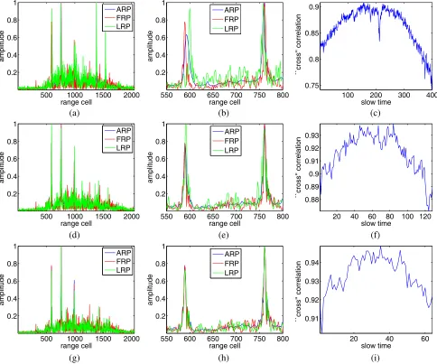
Figure 3. Cross-correlation of range profiles. (a) ARP, FRP and LRP of entire 400 returns; (b) Magnified; (c) Cross-correlation with 400 returns; (d) ARP, FRP and LRP of the first 128 returns; (e) Magnified; (f) Cross-correlation with 128 returns; (g) ARP, FRP and LRP of the first 64 returns; (h) Magnified; (i) Cross-correlation with 64 returns.

quality in the presence of MTRC. In what follows, we will demonstrate this with the range proﬁles shown in Fig. 2.

To make comparisons, ARP, first range profile (FRP) and last range profile (LRP) of the entire 400 returns are illustrated in Fig. 3(a). A part of magnified Fig. 3(a) is shown in Fig. 3(b), it is clear that MTRC cannot be ignored. There are two strong scatterers in the magnified part. The locations of the two scatterers in FRP are totally different with that in LRP. For the left scatterer, the point spread function (PSF) on FRP is on the left of the PSF on LRP, while it is opposite for the right scatterer. Furthermore, the cross-correlation of each range profile with ARP is less than 0.9, shown in Fig. 3(c), which indicates that the algorithm in [8] is not effective in this case.

(6)

When 64 range proﬁles were used, the locations of the two strong scatterers on FRP coincide with each other for ARP and LRP well, which means that the MTRC eﬀect is negligible. What’s more, the cross-correlation increases again as expected, which are shown in Figs. 3(g), (h), (i).

4. ROBUST SUB-INTEGER RANGE ALIGNMENT BASED ON ENTROPY CRITERION

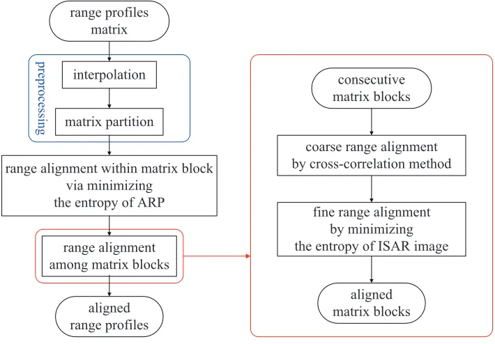
The analyses in Section 3 enlighten us to improve the algorithm in [8]. For the sake of clarity, the proposed algorithm ﬂowchart is shown in Fig. 4. The proposed range alignment algorithm can be divided into three steps. In particular, the ﬁrst step is preprocessing, including the interpolation and matrix partition. The second step is range alignment within each matrix block, and the third step is the range alignment among matrix blocks. These steps will be described in detail in the following.

range profiles matrix

interpolation

matrix partition

range alignment within matrix block via minimizing

the entropy of ARP

range alignment among matrix blocks

aligned range profiles

fine range alignment by minimizing the entropy of ISAR image

coarse range alignment by cross-correlation method

consecutive matrix blocks

preprocessing

aligned matrix blocks

Figure 4. Flowchart of the proposed algorithm.

4.1. Preprocessing

The original range proﬁles are preprocessed for the sake of the following range alignment. The preprocessing procedure can be described as follows.

1) Construct aM×N matrix with the original range proﬁles. M is the number of coherent processing pulses, whileN is number of the sampling points.

2) Interpolation. Each of the range profiles is interpolated to remove the limitation of integer range resolution cell shifting. LetNf denote the interpolation multiple, and then theM×N matrix in the first step becomes theM×N0 matrix, whereN0 =Nf ·N. The precision of range alignment will beρr/Nf. The larger Nf can improve the precision, while increasing the amount of computation. Hence, the choice ofNf should balance the efficiency and precision.

(7)

4.2. Range Alignment within Matrix Block

For each matrix block, MTRC is slight and negligible, hence the range proﬁles in the matrix block can be aligned well by the algorithm proposed in [8]. The ﬁnal range shift Δfmis divided by the interpolation multipleNf, i.e., Δfm= Δm/Nf. The sub-integer range shift is carried out in the frequency domain,

sm(fi+ Δfm) =F T

IF T[sm(fi)] exp

j2πΔf_mt

(15)

whereF T(·) and IF T(·) represent the Fourier transform and inverse Fourier transform, respectively.

4.3. Range Alignment among Matrix Blocks

As clarified in the Introduction, the previously published range alignment algorithms adopt the similarity of adjacent range profiles as the criterion. In the existence of severe MTRC, the similarity between adjacent range profiles no longer holds. This is also true for ARPs of adjacent matrix blocks, shown in Fig. 5. The range profiles matrix in Fig. 2 is partitioned into four matrix blocks. The first three matrix blocks contain 128 range profiles while the forth one contains the rest 16 range profiles. The ARPs of the matrix blocks are calculated according to (11). The original and magnified ARPs are displayed in Fig. 5(a) and Fig. 5(b), respectively. The cross-correlation curve with respect to the shift range cell number shown in Fig. 5(c) is calculated using ARPs of the first two matrix blocks. From Fig. 5(c), we can see that the curve does not show a spike when aligned. The misalignment may occur when using the criteria based on the similarity. Hence, new quality indicator should be developed.

500 1000 1500 2000 0.2

0.4 0.6 0.8 1

range cell

amplitude

1 2 3 4

550 600 650 700 750 800 0.2

0.4 0.6 0.8 1

range cell

amplitude

1 2 3 4

-5 0 5

0.55 0.56 0.57 0.58

shift number

cross-correlation

(a) (b) (c)

Figure 5. ARPs. (a) ARPs; (b) Magniﬁed; (c) Cross-correlation of the ﬁrst two APRs.

The Shannon entropy is used to denote the focal quality of the ISAR image [14]. Suppose that the ISAR image matrix is Iand hasM columns and N rows, then the entropy can be deﬁned as

H=−

M

i=1

N

j=1

|I(i, j)|2

I0

ln|I(i, j)| 2

I0

(16)

where

I0=

M

i=1

N

j=1

|I(i, j)|2 (17)

The lower the entropy is, the better focused the ISAR image is. Since the SNR of the ISAR image can be improved by cross-range imaging, the evaluation of the ISAR image by entropy is more robust. A well focused ISAR image can be achieved only when the range proﬁles are aligned accurately. Thus, the image entropy can be employed to reﬂect the quality of range alignment.

Recall the ﬂowchart in Fig. 4, the red diagram in the right shows the main step. The initial estimated range shift Δ_m of the mth matrix block is calculated via maximizing the cross-correlation of ARPs.

Δm= arg max

Δm

|sm−1

(8)

Because the similarity is weak, misalignment error may occur. Obviously, we should try to decrease the misalignment error to achieve a better range alignment result. Next, a grid search method based on ISAR image entropy is applied to implement a fine range alignment. The search step is set as β =ρr/Nf. The discrete values in the closed interval [Δm−aβ,Δm+aβ] are chosen as candidates to update the initial estimation Δ_m. The values Δ_m+dβ, d ∈ {−a,−a+ 1, . . . , a} are employed to shift the range profiles in themthmatrix block in sequence. Afterwards, phase adjustment algorithm in [16] is applied to the range profiles in the former m matrix blocks. Thus a series of ISAR images can be obtained. The value Δ_m+dβ corresponding to the ISAR image which has the minimum entropy is utilized to update the initial value Δm. By now, all the range profiles are accurately aligned. We can perform the phase adjustment and RD imaging.

5. EXPERIMENTAL RESULTS AND ANALYSIS

5.1. Simulated Data Test

Here, three numerical experiments are performed to demonstrate the performance of the proposed algorithm against MTRC. For comparison, the experiments are also conducted using the algorithms in [8] and that in [6], which are called A1 and A2 for short.

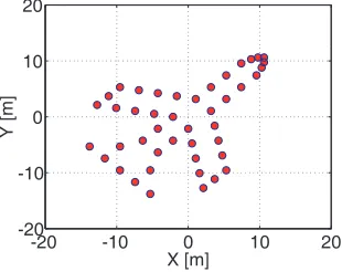
In the simulations, a plane model is assumed to be the target, which is composed of 44 ideal point scatterers with equal magnitude, shown in Fig. 6. The target, at an initial radial distance of 200 km, is moving towards the radar.

The simulation parameters are presented in Table 1. From Experiment A to Experiment C, the resolution is improved along with the increased bandwidth. The range resolution ρr is 0.15 m, 0.075 m and 0.05 m, respectively. The increasing ratioωM T /ρr indicates a severer MTRC. The reference range

-20 -10 0 10 20

X [m]

Y [m]

Figure 6. Sketch map of the target model.

Table 1. Simulation parameters.

PARAMETER VALUE

Experiment A Experiment B Experiment C

Radar parameters

fc 10 GHz 16 GHz 35 GHz

B 1 GHz 2 GHz 3 GHz

Tp 100µs

P RF 1000

M 1024

Target parameters ω 0.0977 rad/s 0.1221 rad/s 0.0837 rad/s

V 50 m/s

(9)

200 400 600 800 1000 4

5 6 7

slow time

range error/range cell

200 400 600 800 1000 −1.5

−1 −0.5 0 0.5 1

slow time

200 400 600 800 1000 −6

−5.8 −5.6 −5.4 −5.2

slow time

range cell

200 400 600 800 1000 450

500

550

600

650

700

slow time

range cell

200 400 600 800 1000 450

500

550

600

650

700

slow time

range cell

200 400 600 800 1000 450

500

550

600

650

700

cross range/m

range/m

−20 0 20

−20

−10

0

10

20

−40 −30 −20 −10 0

cross range/m

range/m

−20 0 20

−20

−10

0

10

20

−40 −30 −20 −10 0

cross range/m

range/m

−20 0 20

−20

−10

0

10

20

−40 −30 −20 −10 0

(a) (b) (c)

(d) (e) (f)

(g) (h) (i)

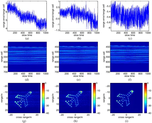
Figure 7. ISAR images of Experiment A. (a) Alignment error curve by A1; (b) Alignment error curve by A2; (c) Alignment error curve by the proposed algorithm; (d) Aligned range profiles by A1; (e) Aligned range profiles by A2; (f) Aligned range profiles by the proposed algorithm; (g) RD image by A1; (h) RD image by A2; (i) RD image by the proposed algorithm.

deviation is distributed uniformly on the interval [−1.5 m, 1.5 m]. The SNR of range profiles is set to 5 dB. For each experiment, 100 Monte Carlo trials are carried out. The results obtained in the first trial of each experiment are shown in Fig. 7–Fig. 9. In the process of the proposed algorithm, the range profile matrix is partitioned into 8 matrix blocks, all of which contain 128 range profiles.

From Fig. 7(a), the absolute alignment error by A1 mainly ranges from 4 range resolution cells to 7 range resolution cells, i.e., the maximum relative alignment error is as much as 3 range resolution cells. As shown in Fig. 7(b), the maximum relative alignment error by A2, 2.5 range resolution cells, is a little smaller than that of A1. Meanwhile, the maximum relative alignment error by the proposed algorithm is only 1 range resolution cell in Fig. 7(c). The aligned range proﬁles by the three methods are shown in Figs. 7(d), (e), (f). As a result, the aligned range proﬁles by the proposed algorithm are much better than that by A1 and A2. The horizontal stripes caused by the range alignment error can be observed from the target images as shown in Fig. 7(g) and Fig. 7(h), which represent the defocusing. The ISAR image by the proposed algorithm is much more clear and is the best focused among the three ones.

(10)

200 400 600 800 1000 -12

-10 -8

slow time

200 400 600 800 1000 -6

-4 -2 0

slow time

200 400 600 800 1000 -16.5

-16 -15.5 -15 -14.5

slow time

range cell

200 400 600 800 1000 400

500

600

700

800

slow time

range cell

200 400 600 800 1000 400

500

600

700

800

slow time

range cell

200 400 600 800 1000 400

500

600

700

800

cross-range/m

range/m

-20 0 20

-20

-10

0

10

20

cross-range/m

range/m

-20 0 20

-20

-10

0

10

20

-40 -30 -20 -10 0

cross-range/m

range/m

-20 0 20

-20

-10

0

10

20

-40 -30 -20 -10 0

(a) (b) (c)

(d) (e) (f)

(g) (h) (i)

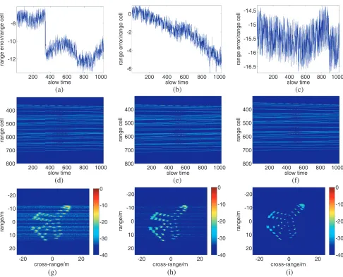
Figure 8. ISAR images of Experiment B. The organization of the ﬁgure is the same as that of Fig. 7.

Similar conclusion can be drawn from the imaging results of Experiment B and Experiment C. As expected, the images by A1 and A2 suﬀer from misalignment and the defocusing is obviously noted from the horizontal stripes. On the contrary, the images obtained by the proposed approach are satisfactory. From Experiment A to Experiment C, the signal bandwidth becomes larger, and then MTRC becomes severer. It can be seen from Fig. 7–Fig. 9 that the performance of A1 and A2 degrades as the bandwidth increases, and the resultant ISAR images are blurred. In contrast, the proposed algorithm is robust against the MTRC. The high-quality ISAR images can still be obtained using the proposed algorithm.

For each trial, the entropy of ISAR image is calculated according to (16) to measure the quality of target image quantitatively. The entropy curves of the three experiments are depicted in Fig. 10. For each Experiment, as we can see, the entropies of the images obtained by the proposed algorithm have the lowest entropy among the three algorithms throughout the 100 Monte Carlo runs. This indicates that the images by the proposed algorithm are the most focused.

5.2. Real-World Data Test

(11)

200 400 600 800 1000 -19 -18 -17 -16 -15 -14 slow time

200 400 600 800 1000 -4 -3 -2 -1 0 1 slow time

200 400 600 800 1000 -14 -13.5 -13 -12.5 -12 -11.5 slow time

slow time

range cell

200 400 600 800 1000 300 400 500 600 700 800 900 slow time range cell

200 400 600 800 1000 300 400 500 600 700 800 900 cross-range/m range/m

-20 0 20

-20 -10 0 10 20 -40 -30 -20 -10 0 cross-range/m range/m

- 20 0 20

-20 -10 0 10 20 -40 -30 -20 -10 0 cross-range/m range/m

-20 0 20

-20 -10 0 10 20 -40 -30 -20 -10 0

(a) (b) (c)

(d) (e) (f)

(g) (h) (i)

Figure 9. ISAR images of Experiment C. The organization of the ﬁgure is the same as that of Fig. 7.

20 40 60 80 100

8 8.5 9 9.5 10 10.5 number entropy A1 A2 Proposed

20 40 60 80 100

(a) (b) (c)

Figure 10. Entropy curve of ISAR images. (a) Experiment A; (b) Experiment B; (c) Experiment C.

(12)

slow time

range cell

100 200 300 400 500 100 200 300 400 500 slow time range cell

100 200 300 400 500 100 200 300 400 500 doppler cell range cell

100 200 300 400 500 100

200

300

400

500 ₄₀

30 20 10 0 doppler cell range cell

100 200 300 400 500 100

200

300

400

500 ₄₀

100 200 300 400 500 100

200

300

400

500 ₄₀

30 20 10 0

(a) (b) (c)

(d) (e) (f)

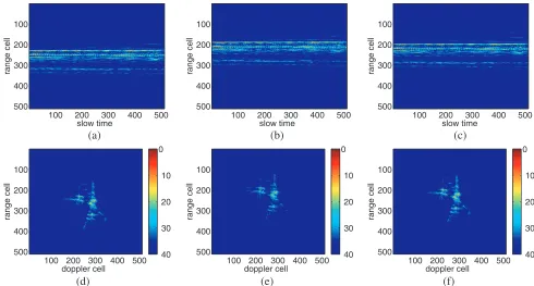
Figure 11. ISAR Images of segment 1. (a) Aligned range profiles by A1; (b) Aligned range profiles by A2; (c) Aligned range profiles by the proposed algorithm; (d) RD image by A1; (e) RD image by A2; (f) RD image by the proposed algorithm.

slow time

range cell

100 200 300 400 500 100 200 300 400 500 slow time range cell

100 200 300 400 500 100 200 300 400 500 doppler cell range cell

100 200 300 400 500 100

200

300

400

500 ₄₀

100 200 300 400 500 100

200

300

400

500 ₄₀

100 200 300 400 500 100

200

300

400

500 ₄₀

30 20 10 0

(a) (b) (c)

(d) (e) (f)

(13)

From the ISAR images, it is clear that the proposed algorithm is able to get the most focused ISAR images due to the most accurate range alignment, which validates the performance of the algorithm.

Table 2 gives the entropies of the ISAR images obtained using real data. The entropy of the ISAR image obtained by the proposed algorithm is the lowest among the three ones. Since MTRC is slightly, the improvement is not signiﬁcant as that concluded in the simulation.

Table 2. Entropies of ISAR images.

echos A1 A2 Proposed

segment 1 7.5608 8.0133 7.4134 segment 2 7.8711 8.2163 7.7079

In the following, we use the range proﬁles of segment 2 to evaluate the anti-noise performance of the proposed algorithm. The mean value of ISAR image entropy is calculated over 50 Monte Carlo simulations under each SNR condition and the result is depicted in Fig. 13. The SNR is set from−3 dB to 12 dB with a step of 3 dB by adding complex Gaussian white noises into the original range proﬁles. The entropy decreases as SNR increases. Compared with A1 and A2, the proposed method is capable of generating the ISAR image with the minimum entropy. Caused by matrix partition. the advantage of the proposed algorithm is whittled away gradually as SNR decreases. Hence, the issue of range alignment under low SNR need to be studied in the future.

0 5 10

8 9 10 11 12

SNR/dB

Entropy Mean

A1 A2 Proposed

Figure 13. Entropy mean of ISAR images of segment 2 with respect to SNR.

5.3. Computational Complexity Analysis

In this subsection, the computation burdens of the proposed method and A1 are numerically analyzed. Previous sections show that the two methods are performed in an iteration manner. Suppose the number of range cells and pulses isN and M, respectively.

For A1, let P1 denote the number of iterations, thus the numbers of complex multiplications and complex additions can be formula as

NmulA1 =

2(M + 1)N

2 log2N + 2(M + 1)N

P1 (19)

N_addA1 =

2(M + 1)Nlog₂N + (M+ 1)N

P1 (20)

(14)

range alignment iterations and number of phase adjustment iterations, respectively. Then, the total computation burden of the proposed method is about

N_mulP roposed =

2(M+ 1)N0

2 log2N0+ 2(M + 1)N0

P2+Nm

+ 1

2 (M Nlog2M+ 4M N)Q (21)

N_addP roposed =

2(M+ 1)N0log2N0+ (M+ 1)N0

P2+Nm

+ 1

2 (2M Nlog2M+ 2M N)Q (22) In practice, P1 ≈P2≈10 andQ≈100. With regard to the range proﬁles of segment 2 in the last subsection, N =M = 512, N0= 8N and Nm = 4. Hence,

N_mulP roposed

NA1

mul

= 39.67 (23)

N_addP roposed

N_addA1 = 36.79 (24)

The execution time on personal computer of A1 is 0.90 s, and that of the proposed algorithm is 37.67 s. As we can see, the mathematical analysis agrees with the process time results. The proposed algorithm is less eﬃcient than A1 but acceptable.

6. CONCLUSIONS

To conclude, a robust range alignment method against MTRC has been proposed. Robust range alignment against MTRC was developed by minimizing the entropy of ARP and ISAR image. Moreover, the proposed range alignment algorithm achieved a breakthrough of the limit of integer range resolution cell by interpolating the range proﬁles. Both simulated and real-world data experiments were exploited to show the advantages of the proposed approach. The work and results can be helpful for achieving highly focused ISAR image.

In addition, the proposed method was not aﬀected by how the pulse compression is achieved, and it could deal with both the dechirped process and matched-ﬁlter-based pulse compression.

For targets with complex motion or under low SNR condition, however, range alignment is much more involved, which will be studied in future work.

ACKNOWLEDGMENT

This work was supported by the National Natural Science Foundation of China under Grant 61471373. The authors would like to thank all the editors and reviewers for their valuable comments to improve the quality of the paper. They would also like to thank Dr. Liu Y. for his kind guidance and great help in revising the manuscript.

REFERENCES

1. Chen, C. C. and H. C. Andrews, “Target-motion-induced radar imaging,” IEEE Trans. Aerosp. Electron. Syst., Vol. 16, No. 1, 2–14, 1980.

2. Martorella, M., E. Giusti, A. Capria, et al., “Automatic target recognition by means of polarimetric ISAR images and neural networks,”IEEE Trans. Geosci. Remote Sens., Vol. 47, No. 11, 3786–3794, 2009.

3. Musman, S., D. Kerr, and C. Bachmann, “Automatic recognition of ISAR images,” IEEE Trans. Aerosp. Electron. Syst., Vol. 35, No. 4, 1240–1252, 1999.

4. Yan, X., J. Hu, G. Zhao, J. Zhang, and J. Wan, “A new parameter estimation method for GTD model based on modiﬁed compressed sensing,” Progress In Electromagnetics Research, Vol. 141, 553–575, 2013.

(15)

6. Munoz-Ferreras, J. M. and F. Perez-Martinez, “Subinteger range-bin alignment method for ISAR imaging of noncooperative targets,”EURASIP J. Adv. Signal Process., Vol. 2010, 1–16, 2010. 7. Yuan, B., S. Y. Xu, and Z. P. Chen, “Translational motion compensation techniques in ISAR

imaging for target with micro-motion parts,” Progress In Electromagnetics Research M, Vol. 35, 113–120, 2014.

8. Zhu, D. Y., L. Wang, Y. S. Yu, et al., “Robust ISAR range alignment via minimizing the entropy of the average range proﬁle,” IEEE Geosci. Remote Sens. Lett., Vol. 6, No. 2, 204–208, 2009. 9. Wang, G. Y. and Z. Bao, “A new algorithm of range alignment in ISAR motion compensation,”

Acta Electronica Sinica, Vol. 26, No. 6, 5–8, 1998.

10. Wang, J. F. and D. Kasilingam, “Global range alignment for ISAR,”IEEE Trans. Aerosp. Electron. Syst., Vol. 39, No. 1, 351–357, 2003.

11. Steinberg, B. D., “Microwave imaging of aircraft,”Proceedings of the IEEE, Vol. 16, No. 12, 1578– 1592, 1988.

12. Ye, C. M., J. Xu, Y. N. Peng, et al., “Performance analysis of Doppler centroid tracking for ISAR autofocusing,”Acta Electronica Sinica, Vol. 37, No. 6, 1324–1328, 2009.

13. Jackowatz, C., D. Wahl, P. Eichel, et al., Spotlight-mode Synthetic Aperture Radar: A Signal Processing Approach, Kluwer Academic Publishers, Boston, 1996.

14. Zhang, L., J. L. Sheng, J. Duan, et al., “Translational motion compensation for ISAR imaging under low SNR by minimum entropy,” EURASIP J. Adv. Signal Process., Vol. 2013, 1–19, 2013. 15. Li, X., G. S. Liu, and J. L. Ni, “Autofocusing of ISAR images based on entropy minimization,”

IEEE Trans. Aerosp. Electron. Syst., Vol. 35, No. 4, 1240–1252, 1999.

16. Qiu, X. H., A. H. W. Cheng, and Y. S. Yam, “Fast minimum entropy phase compensation for ISAR imaging,”Journal of Electronics and Information Technology, Vol. 26, No. 10, 1656–1660, 2004. 17. Xu, G., M. D. Xing, L. Yang, et al., “Joint approach of translational and rotational phase error

corrections for high-resolution inverse synthetic aperture radar imaging using minimum-entropy,”

IET Radar Sonar Navig., Vol. 10, No. 3, 586–594, 2016.

18. Martorella, M., J. Palmer, F. Berizzi, et al., “Polarimetric ISAR autofocusing,”IET Signal Process., Vol. 2, No. 3, 312–324, 2008.

19. Zhang, S. H., Y. X. Liu, and X. Li, “Fast entropy minimization based autofocusing technique for ISAR imaging,”IEEE Trans. Signal Process., Vol. 63, No. 13, 3425–3434, 2015.

20. Martorella, M., F. Berizzi, and B. Haywood, “Contrast maximisation based technique for 2-D ISAR autofocusing,”IEE Proceedings: Radar Sonar Navig., Vol. 152, No. 4, 253–262, 2005.

21. Xing, M. D., R. B. Wu, and Z. Bao, “High resolution ISAR imaging of high speed moving targets,”

IEE Proceedings: Radar Sonar Navig., Vol. 152, No. 2, 58–67, 2005.