Optimization Design Methodology of Miniaturized Five-Band
Antenna for RFID, GSM, and WiMAX Applications
Ayia A. S. A. Jabar and Dhirgham K. Naji*
Abstract—This paper presents a novel design methodology for the design and optimization of a miniaturized multiband microstrip patch antenna (MPA) for wireless communication systems. Two design steps are used to do that. In the first step, an initial antenna is designed by a trial and error approach to operate nearly in the desired frequency bands, but the level of impedance matching (s11 <−10 dB) for one or more bands is unsatisfactory, or some bands are uncovered by the antenna. The second design step is used after that to achieve optimized antenna by applying an optimization algorithm to effectively fine-tune the impedance matching of the initial deigned antenna to closely satisfy all the desired frequency bands. As an illustrative example, the proposed optimization methodology is used for designing a miniaturized multiband MPA suitable for operating at five different frequency bands, 915 MHz (RFID band), 1850 MHz (GSM band), (ISM — Industrial, Scientific, Medical), 2.45 and 5.8 GHz, and 3.5 GHz (WiMAX band). The proposed MPA used here is composed of two patch structures printed on both sides of an FR4 substrate occupying an overall size of just 28×28 mm2. The final optimized antenna is fabricated, and its simulated and measured results are coinciding with each other validating the design principle. Moreover, simulation antenna performance parameters, surface current distribution, realized peak gain, and efficiency besides the radiation patterns at the desired frequency bands are obtained using CST MWS.
1. INTRODUCTION
In recent years, much interest has been paid to the study and design of multiband antennas for use in mobile communication systems covering all the desired frequency bands needed by international standard. Due to the limited space for these applications, designing a multiband antenna having satisfactory performance is a challenging task. Miniaturized antennas with multiband characteristic for mobile wireless applications, such as internet of things [1–4], wireless sensor networks [5], wearable devices [6, 7], RFID portable devices [8–12], and implantable biomedical systems [13, 14], have become urgent requirements. Over the past decade, various methods and optimization techniques have been introduced for multiband or wideband antenna design. Some of the most commonly used techniques for solving different electromagnetic problems particularly antenna design are agenetic algorithm (GA) [15–21], simulated annealing (SA) [22, 23], invasive weed optimization (IWO) [24–26], and particle swarm optimization (PSO) [27–33]. The proposed antennas presented in these papers clarify the advantages of PSO algorithm such as easy implementation and suitability for use in the design of those optimized antennas including single- and multi-objective optimization problems compared with other aforementioned techniques GA, SA, and IWO.
Antenna optimization is greatly dependent on an efficient objective function that leads to an optimizer for getting desirable solution in the visible region. Generally in the literature, two
Received 29 January 2019, Accepted 14 March 2019, Scheduled 27 March 2019
* Corresponding author: Dhirgham Kamal Naji ([email protected]).
conventional objective functions (F) to be minimized, namely, F1 = max(|S11(f)|) [22, 27, 28, 33] and
F2 = sum(|S11(f)|dB) [15, 16, 20, 21, 23], wheref is the sample frequency ranging fromfminto fmax, are used for designing a multiband antenna. The objective functions F1 and F2 are minimized for getting an improvement in |S11(f)| and the area under |S11(f)|dB, respectively for the all sample frequencies resulting in an antenna having wide or multiband characteristic [34].
In general, two well-known methods are recently available for solving multi-objective optimization problems: (1) Pareto dominance (PD) [30, 35, 36] and (2) conventional weighted aggregation (CWA) [15, 16, 20–29]. In a PD method, all competing single-objective functions for the optimization problem can be simultaneously dealt with by the designers through deriving complete Pareto front (PF) that exposes the compromise between those objectives resulting in miscellaneous representations of the optimal solutions. Whatever, although PD methods are suitable for solving multi-objective optimization problems particularly for antenna design, for many problems, large number of iterations and optimization calculations are required. A complete PF must be obtained, especially in problems that contain many design targets and antenna geometrical parameters. On the other hand, in a CWA approach, a number of discrete weighting coefficients of single-objective functions are added to constitute the objective function that allows all single-objective functions to be minimized simultaneously. This method is simple to be implemented for antenna optimization problems by properly finding the convenience aggregation of weighting coefficients for the assortment of single-objective functions. Also, the CWA approach is especially easy in optimization problems when the desired objectives are related or use same physical units [37] such as the multi-objective function for the designed antenna presented in this work.
In this paper, a novel optimization objective function is proposed for designing multiband antenna under the constraint of miniaturized size. This objective function for the first time deals with both the lower and higher frequencies that belong to the all desired frequency bands. In this work, the PSO kernel implemented in MATLAB and finite integration technique (FIT) offered by CST Microwave Studio (MWS) are operated in parallel to evaluate the objective function. As an illustrative example, a five-band antenna is optimized to cover the desired bands allocated for sub-6 GHz applications: 915 MHz and 2.45/5.8 GHz for RFID, 1850 MHz for GSM, 2.4/5.8 GHz for WLAN, and 3.5 GHz for WiMAX. The designed antenna is verified experimentally.
2. PROPOSED OPTIMIZATION METHODOLOGY
To find the best solution that treats a certain problem, optimization technique is used. The optimization of geometric parameters for any application-based microwave/RF device becomes very crucial since the device is necessary to exhibit a particular desired response. For optimizing the microwave designs, Evolutionary Algorithms (EAs) involve GA, PSO, SA, and IWO which have been used as very reliable methods. These EA algorithms can be used to optimize many parameters simultaneously, and they overcome the local minima problems in most of the cases. Compared to other EAs techniques such as GA, SA, and IWO, the PSO algorithm is much easier to understand and implement, and requires the least mathematical preprocessing. Therefore, it is well adopted here to be used in the design optimization of the proposed antennas.
The procedure of PSO optimization resembling the social behavior of a swarm of bees while searching for the region with most flowers. It is based on a population of particles that fly in space with velocity dynamically adjusted according to its own flying experience and the flying experience of the best among the swarm. Each potential solution in the PSO algorithm is represented as a particle with a position vector ofx= (x1x2, . . . , xN) and velocityv= (v1v2, . . . , vN) in anN-dimensional optimization. An associated value for each particle, at each time step, is evaluated according to an objective function which is critically configured with a consideration of the search objective. In the PSO, it is firstly generating a population of Np particles at random to search a broad population of possible solution in the entire search space. Generally, using a defined objective function, for all particles the objective values are evaluated, and the global best (xbest) and personal best (xbesti ) are calculated which are used in producing the new position xi+1 and new velocity vi+1 for each particle after each iteration i+ 1. Thus, at iterationi+ 1,vi+1 and xi+1 for each particle are updated by:
vi+1 = ωvi+ 2η1
xbesti −xi
+ 2η2
xbest−xi
xi+1 = xi+vi+1 (2)
In Eq. (1), the time varying parameterω, which is called inertia factor, decreases with iteration number from a maximum value at the first iteration and goes to a minimum at the last iteration. Two statistically independent random variablesη1andη2, both uniformly distributed in the interval [0,1], are introduced to stochastically vary the relative pull of the personal and global best particles. The designs are optimized PSO integrated with CST Microwave Studio.
Mathematically, the nonlinear global optimization problem to be solved in this work is defined as: Find the set x = (x1x2, . . . , xN) of Ng geometrical antenna parameters that will optimize the function
Minimize F(x) (3a)
subject to h(x) = 0, g(x)≤0 (3b)
and the constraints : xli ≤xi ≤xui i= 1,2, . . . , Ng,
where F(x) described in Eq. (3) is the objective function, h(x) the equality constraint, g(x) the inequality constraint, and x the vector of design variables. Also, xli and xui are the lower and upper bounds on the N design variables, respectively.
The goal for using PSO considered here was aimed to achieve optimized antenna by tuning CST simulated frequency bands to the counterpart desired bands by altering the initial designed antenna geometrical parameters within allowed prescribed ranges. A suitable optimization model to satisfy this aim is:
Minimize F(x) =−1
2[F1+F2 +. . .+Fk],
=−1 2
K
i=1
Fi, i= 1,2,3, . . . , K (4a)
Subject to Aopt =Aref (4b)
and the constraints : xli ≤xi≤xui i= 1,2, . . . , Ng,
In this model, Aopt and Aref represent area of the optimized antenna and the reference antenna, respectively.
At the jth band (1≤j ≤K):
Fj =WLjELj+WHjEHj (5)
where
ELj = U
−fLj+fdLjmax
+UfLj−fdLjmin
(6a)
EHj = U
−fHj+fdHjmax
+UfHj−fdHjmin
(6b)
and
WLj = fdLjmin
fLj (7a)
WHj = fHj fmax
dHj
(7b)
fLj = f
S11 at fLj =−10 dB dS11
df =−1
(8a)
fHj = f
S11 at fHj =−10 dB dS11
df = +1
S11 at fLj = 20 log
Zin at fLj −Zo
Zin at fLj +Zo
(dB) (9a)
S11at fHj = 20 log
Zin at fHj −Zo Zin at fHj +Zo
(dB) (9b)
In the objective function above, Eq. (6), U refers to the unit step function whileELj and EHj denote, respectively, the error of thejth −10-dBS11 impedance bandwidth (BWj =fHj−fLj) wherefLj and fHj denote, respectively, the jth lower and higher frequencies. In Eq. (9), S11at fLj, S11at fHj and Zin at fLj,Zin atfHj refer, respectively, to the return loss and the input impedance of the antenna atfLj, fHj, and Zo is the characteristic impedance (Zo = 50 Ω). The symbols WLj and WHj represent the weighting coefficients corresponding to thejth error functions ELj and EHj, respectively, andK refers to the number of desired frequency bands. The ‘+’ sign in F(x) is a logic “AND” addition, and the values of ELj and EHj are either logic ‘1’ or logic ‘0’. Thus, for each calculated jth frequency band BWj to be greater than the jth desired band (BWdj = fdHj−fdLj), ELj and EHj are equal to one, and otherwise they are equal to zero, wherefdHj andfdLj are thejth desired high and low frequencies, respectively. On the other hand, the ranges of weighting coefficients WLj and WHj are, respectively, (fdLjmin/fdLjmax)≤WLj ≤1 and (fdHjmin/fdHjmax)≤WHj ≤1. To easily understand the concepts of Eqs. (4)–(9), see the following two comments.
a) The error ofjth lower frequency ELj=U(−fLj+fdLjmax) +U(fLj−fdLjmin) where the first term is
U−fLj+fdLjmax
=
1, fLj ≤fdLjmax 0, fLj > fdLjmax
, (10a)
and the second term is
UfLj−fdLjmin
=
1, fLj ≥fdLjmin
0, fLj < fdLjmin . (10b)
Thus, if both terms of ELj are equal to 1, then ELj = 2, which means that fdLjmin≤fLj ≤fdLjmax, or thejth lower frequencyfLj is satisfied to range between the minimum and maximum values of the jth desired lower frequency fdLjmin and fdLjmax, respectively.
b) In the same manner, the error of thejth higher frequencyEHj =U(−fHj+fdHjmax) +U(fHj−fdHjmin), where its first term is
U−fHj+fdHjmax
=
1, fHj ≤fdHjmax
0, fHj > fdHjmax , (11a)
and the second term is
UfHj −fdHjmin=
1, fHj ≥fdHjmin
0, fHj < fdHjmin (11b)
Thus, if both terms ofEHj are equal to 1, then EHj = 2, which means that fdHjmin ≤fHj ≤fdHjmax, or the jth higher frequency fHj is satisfied to range between the minimum and maximum values of the jth desired higher frequency fdHjmin and fdHjmax, respectively. As a result, if all the bands (i= 1,2, . . . , K) are satisfied,F(x) will be at a minimum value given by:
F(x) =
⎧ ⎪ ⎨ ⎪ ⎩
−K, if WLi=WHi= 1
−K K
i=1
(WLi+WHi), if WLi= 1 and WHi= 1 , i= 1,2, . . . , K (12)
Input the Desired Frequency Bands and the Initialized Antenna Geometrical Parameters
Area of the optimized antenna: A
Number of frequency bands: K
For each -10 dB-S11jth frequency band (1 ≤j ≤ K ), specify the following parameters: -Lower frequency for each band: f , f , ..., f .
-Higher frequency for each band: f , f , ..., f .
-minimum desired Lower frequency: f , f , ..., f .
-minimum desired Higher frequency: f , f , ..., f .
PSO Initialization
Specify geometrical antenna parameter size that entering the optimization process : N .
Determine particle size : N = 3N or 5N .
Initialize PSO particles’ positions within the lower and upper bounds on the N design variables :
Lower and Higher Frequencies Evaluation
For each -10 dB-S11jth frequency band (1 ≤j ≤ K): - Applying Eqs. (8a) and (9a) for f , f , ..., f .
- Applying Eqs. (8b) and (9b) for f , f , ..., f .
Weighting Coefficients Evaluation
For each -10 dB-S11jth frequency band (1 ≤j ≤ K):
- Applying Eq. (7a) for W , W , ..., W .
- Applying Eq. (7b) for W , W , ..., W .
Lower and Higher Errors Evaluation
For each -10 dB-S11jth frequency band (1 ≤j ≤ K): - Applying Eq. (6a) for E , E , ..., E .
- Applying Eq. (6b) for E , E , ..., E .
Objective Function Evaluation
For each -10 dB-S11jth frequency band (1 ≤j ≤ K): - Applying Eq. (5) for F , F , ..., F .
Applying Eq. (4) for evaluating F(x).
.
.
.
.
.
.
.
.
.
.
opt
L1 L2 Lj
H1 H2 Hj
min min min dL1 dL2 dLj
min min min dH1 dH2 dHj
g
p g g
g
x il ≤x i≤ xiu i = 1, 2, ..., N .g
L1 L2 Lj
H1 H2 Hj
L1 L2 Lj
H1 H2 Hj
L1 L2 Lj
H1 H2 Hj
1 2 j
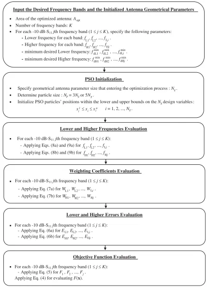
First Block (Input the Desired Frequency Bands and the Initialized Antenna Geometrical Parameters): The optimization model begins by using a trial and error approach for the proposed antenna, which has an overall size of Aref and initialized geometrical parameters for operating nearly throughout some desired frequency bands. In this step, the number of frequency bands K, the area of the optimized antenna Aopt, and for each −10 dB-S11 jth frequency band (1 ≤ j ≤ K): the lower frequencies fL1, fL2, . . . , fLj, higher frequencies fH1, fH2, . . . , fHj, minimum desired Lower frequency fdLmin1, fdLmin2, . . . , fdLjmin, and minimum desired higher frequency: fdHmin1, fdHmin2, . . . , fdHjmin are specified.
Second Block (PSO Initialization): In PSO initialization phase, it is required to specify the number of geometrical antenna parameters entering the optimization process (Ng) and the particle size Np (= 3Ng or 5Ng), in addition to PSO particles’ positions allowed to cover the space search, xl
i ≤xi ≤xui fori= 1,2, . . . , Ng.
Third Block (Lower and Higher Frequencies Evaluation): The goal of the proposed model is for covering all thejth −10 dB-S11frequency bands (1≤j ≤K) by the optimized antenna. Eqs. (8a) and (9a) are used for evaluating fL1, fL2, . . . , fLj, whereas Eqs. (8b) and (9b) are employed for calculating
fH1, fH2, . . . , fHj.
Fourth Block (Weighting Coefficients Evaluation): In this step, for each jth −10 dB-S11 frequency band (1 ≤ j ≤ K), the lower and higher weighting coefficients, WL1, WL2, . . . , WLj, and WH1, WH2, . . . , WHj, are calculated by applying Eqs. (7a) and (7b), respectively.
Fifth Block (Lower and Higher Errors Evaluation): In this step, for each jth −10 dB-S11 frequency band (1 ≤ j ≤ K), the lower and higher errors, EL1, EL2, . . . , ELj, and EH1, EH2, . . . , EHj, are calculated by applying Eqs. (6a) and (6b), respectively.
Sixth Block (Objective Function Evaluation): This is the final step in the optimization model that evaluates the multi-objective function F(x) by applying Eq. (4) with summing the all single-objective functionsF1, F2, . . . , Fj.
3. ANTENNA DESIGN VIA OPTIMIZATION METHODOLOGY
The objective function discussed in the previous section is applied here to design, as an illustrative example, an optimized antenna having multiband characteristic under the constraint of miniaturized size. The concept of two well-known techniques, fractal and spiral geometries because of their main characteristics, multiband and miniaturization, is adopted for designing MPAs using the aforementioned optimization methodology. In this work, the antenna is optimized using two softwares running in parallel, PSO technique implemented under MATLAB environment, while the electromagnetic (EM) part of the objective function was offered by CST Microwave Studio software package. At each iteration of the PSO algorithm, initial designed antenna geometrical parameters are updated to CST MWS to extract the EM simulated result, antenna return lossS11. Then,S11result is mapped again in MATLAB for evaluating the objective function (multiband impedance matching criterion) by the PSO algorithm. This optimization process as shown in Figure 2 is still for running until enough number of iterations is reached, and consequently an optimized antenna with satisfied performance is obtained. Generally, the following two main steps are performed:
1) First Design Step
Calculate Objective
Function, F( x)
Optimal Antenna Geometrical Parameters Is Satisfied
or Enough is
reached ? Design step 1
Generate Initial Antenna
Geometrical Parameters MATLAB
CST MWS
Design step 2
Evaluate the Performance of
the Optimized Antenna Calculate Return
Loss, S
Generate New Antenna Geometrical Parameters Using
PSO Algorith No
Yes 11
F(x)
Np
Figure 2. Data flow for designing both the initialized and optimized antennas. The initial designed antenna geometrical parameters are taken from the optimized antenna.
2) Second Design Step
In this step, the procedure presented in Section 2 is applied to the initialized antenna. This procedure yields an optimized antenna size ofAopt=Aref and operating over the desired frequency bands by applying Eqs. (4)–(9) for describing the objective function.
3.1. Initial Design of Fractal- and Spiral-Shaped Patch Antenna
Eqs. (4)–(9), to the initialized antenna structure aiming to cover the appropriate bands. The following sections present in details the description and investigation of the procedure for designing and analyzing the proposed antenna structure that achieves the aforementioned frequency bands under the constraint of miniaturized size.
Figures 3(a)–(d) show the simulation models 3D and 2D besides the front and back sides, respectively of the proposed initial designed antenna, and the front and back sides of the manufactured optimized antenna are depicted, respectively, in Figures 3(e)–(f). The antenna includes two structures printed on both sides of an FR4 substrate with overall dimensions (Lsub×Wsub) of (28 mm×28 mm) with thicknesshsub1.6 mm, relative permittivity r = 4.3, and loss tangent 0.02. A second-order Minkowski fractal-shaped patch strip is printed on the front side of the FR4 substrate, and on its back side a spiral-shaped loop structure is printed.
The fractal-shaped strip patch antenna length and width are, respectively, Lp = 12 mm and Wp = 14 mm, and thicknesstf = 0.5 mm. The spiral width and length are, respectively, Lsp = 22 mm and Wsp = 22 mm, and its thickness ts = 0.5 mm. The spacing between strips d = 5 mm. A 50-Ω SMA is connected to the bottom side of coplanar waveguide (CPW)-feed, with length (Lf = 9 mm) and width (Wf = 2 mm), and another side of the feed line is connected to the fractal patch strip for signal transmission. A linearly tapered ground plane, having a width (W1 = 12.75 mm) and length (Lg = 5 mm), is printed at the gap (g = 0.25 mm) from the CPW-feed line for widening impedance bandwidth.
3.2. Design Procedure of Initialized Antenna
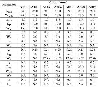
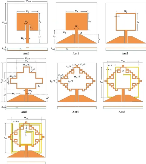
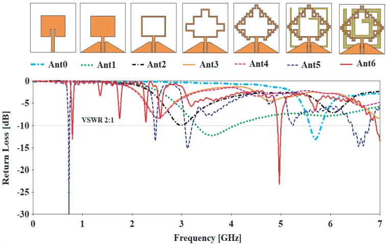
The structural evolution of the proposed initialized designed antenna, which comprises seven design structures, is shown in Figure 4, and the optimized values of those antenna parameters are listed in Table 1. Figure 5 plots the CST simulated return loss (S11) results of the antennas. The design and analysis of these seven structures besides their S11 results will be extensively investigated in the next subsections.
Table 1. The final dimensions of the designed antennas.
parameter Value (mm)
Ant0 Ant1 Ant2 Ant3 Ant4 Ant5 Ant6 Lsub 28.0 28.0 28.0 28.0 28.0 28.0 28.0 Wsub 28.0 28.0 28.0 28.0 28.0 28.0 28.0
hsub 1.5 1.5 1.5 1.5 1.5 1.5 1.5
Lp 12.0 12.0 12.0 12.0 12.0 12.0 12.0
Wp 15.0 14.0 14.0 14.0 14.0 14.0 14.0
Lf 9.0 9.0 9.0 9.0 9.0 9.0 9.0
Wf 2.0 2.0 2.0 2.0 2.0 2.0 2.0
Ls 4.0 NA NA NA NA NA NA
Ws 0.5 NA NA NA NA NA NA
g NA 0.25 0.25 0.25 0.25 0.25 0.25
Lg NA 5.0 5.0 5.0 5.0 5.0 5.0
W1 NA NA 12.75 12.75 12.75 12.75 12.75
t1 NA NA 0.5 0.5 0.5 0.5 0.5
Lsp NA NA NA NA 22.0 22.0 22.0
Wsp NA NA NA NA 22.0 22.0 22.0
W2 NA NA NA NA 5.0 5.0 3.5
t2 NA NA NA NA 0.5 0.5 0.5
(a) (b)
(c) (d)
(e) (f)
Ant0 Ant1 Ant2
Ant3 Ant4 Ant5
Ant6
Figure 4. The evolution design procedure for the proposed antenna.
3.3. Design of the Conventional MPA
Figure 5. Simulated return loss characteristics for antennas.
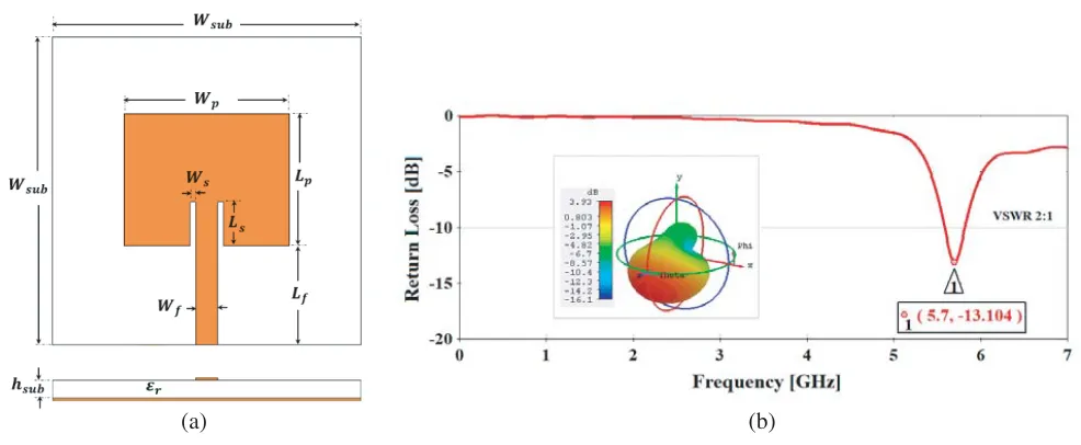
Eqs. (13)–(16) [38], is used to design MPA to operate at the desired resonance frequency fr= 5.8 GHz (RFID/WLAN band) by assuming the relative permittivity εr = 4.3 (FR4) and the height of the substratehsub = 1.6 mm.
εef f = εr+ 1
2 +
εr−1 2
1
1 + 12h/Wp
(13)
where (εr, h, Wp) are the dielectric constant, height of the substrate, and width of the patch, respectively. The patch length and width of the antenna identify antenna resonance. The patch length (Lp) of the antenna for dominant mode resonance is given as:
Lp = 1
2fr
√
εef f√μ0ε0 −
2ΔLp (14)
where,
ΔLp= 0.412h(εef f + 0.300) (εef f −0.258)
Wp
h + 0.262
Wp
h + 0.813
(15)
The width of the patch antenna is given by
Wp= c 2fr
2 εr+ 1
(16)
(a) (b)
Figure 6. (a) Conventional microstrip inset-fed MPA, Ant0 and (b) its return loss and radiation pattern.
3.4. Design of the Tapered CPW-fed MPA
After that conventional MPA (Ant0) was designed to operate atfr = 5.8 GHz, Ant0 is redesigned after replacing its inset fed by the counterpart CPW-fed with the tapered ground plane, and consequently Ant1 is produced as shown in Figure 7(a). As noticed from the S11 plot, Figure 7(b), Ant1 resonates at fr1 ∼= 3.6 GHz with return loss of approximately −12 dB, in addition to fr2 ∼= 5.9 GHz presented in the conventional MPA but with return loss greater than −10 dB. The overall dimension Lsub×Wsub of the antenna is 28 mm×28 mm whereas its patch size Lp×Wp is 12 mm×14 mm.
(a) (b)
Figure 7. (a) Tapered CPW-fed MPA, (Ant1) and (b) its return loss characteristic.
3.5. Design of the Minkowski Fractal Antenna
(a) (b) (c)
Figure 8. Tapered CPW-fed Minkowski fractal antenna (MFA). (a) MFA0. (b) MFA1. (c) MFA3.
The MFA0, as seen in Figure 8(a) is evolved from Ant1 by replacing its patch structure with the counterpart patch strip of thicknesst1 = 0.5 mm. Then, MFA1 is obtained by adding three medium size rectangular strips of length (Lp/3)×(Wp/3) to the right, left, and upper sides of the large rectangular strip of MFA0, see Figure 8(b). After that, MFA2 as depicted in Figure 8(c) can be produced by adding three of small strips with length (Lp/9)×(Wp/9) to the three medium strips of MFA1, and other eight of such small strips are added to its main rectangular strip with two strips for each one of the four sides. The return loss curves of these antennas are plotted in Figure 9. It is seen from this figure that Ant2 (Ant3) resonates at two frequencies 3 GHz and 6 GHz (2.5 GHz and 4.8 GHz) whereas Ant3 resonates at three frequencies, 2.5, 4.5 and 6.6 GHz.
Figure 9. Simulated return loss characteristics for Tapered CPW-fed Minkowski fractal antenna (MFA). (a) MFA0 or Ant2. (b) MFA1 or Ant3. (c) MFA2 or Ant4.
3.6. Design of the Minkowski Fractal- and Spiral-Based Antenna
As discussed in the previous subsection, it is required to add other structure to the designed antenna, MFA2 to operate at multiple frequencies covering the desired bands. The spiral structure is a appropriate solution to do that duo to its ability to add more resonance frequencies to the original designed antenna by sufficiently selecting their geometrical parameters, spiral width and length, Lsp and Wsp, besides its thickness t2, spacing between strips W2, and loop length L1. Figure 10 shows the proposed initial designed antenna after adding the spiral geometry (colored as yellow) in the back side of the FR4 substrate.
(a) (b)
Figure 10. Tapered CPW-fed Minkowski fractal- and spiral-based antenna (MFSA). (a) MFSA1. (b) MFSA2.
Figure 11. Simulated return loss characteristics for Tapered CPW-fed Minkowski fractal- and spiral-based antenna (MFSA).
capable of operating at different frequencies, but these frequencies do not meet the desired frequencies. Thus, it is required to fine-tune these bands obtained from the initial designed antenna (Ant6) by using the optimization design methodology described earlier. The following section discusses in details the application of the design methodology for the initialized designed antenna (MFSA) to yield an optimized antenna having appropriate frequency bands.
4. DESIGN OF THE OPTIMIZED ANTENNA
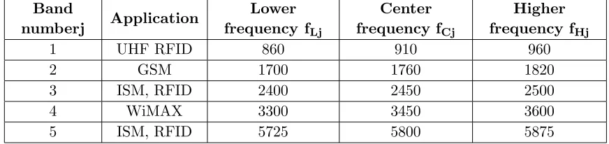
This section presents the application of the objective function described in the previous section to the initial designed antenna for covering the desiredK-frequency bands. For eachjth band (1≤j≤K), the jth lower and higher frequenciesfLj andfHj, respectively, are required to be within the maximum and minimum of lower and higher frequenciesfdLj andfdHj, i.e.,fdLjmin≤fLj≤fdLjmaxandfdHjmin ≤fHj ≤fdHjmax. Tables 2 and 3 illustrate the frequency band used in wireless communications and the counterpart desired bands defined in the optimization methodology, respectively, for five desired bands,K = 5.
Table 2. Frequency bands (in MHz) considered for wireless communications.
Band
numberj Application
Lower frequency fLj
Center frequency fCj
Higher frequency fHj
1 UHF RFID 860 910 960
2 GSM 1700 1760 1820
3 ISM, RFID 2400 2450 2500
4 WiMAX 3300 3450 3600
5 ISM, RFID 5725 5800 5875
Table 3. The desired Frequency bands (in MHz) used in optimization methodology.
Band numberj Lower desired frequency Higher desired frequency fdLj fdLjmin fdLjmax fdHj fdHjmin fdHjmax
1 860 840 860 920 920 940
2 1760 1700 1760 1800 1800 1820
3 2390 2390 2420 2450 2450 2460
4 3300 3000 3300 3600 3600 3800
5 5725 5680 5725 5875 5875 5900
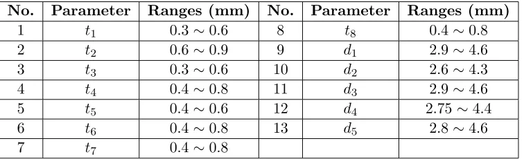
The initialized antenna designed in the previous sections is replotted here, as shown in Figure 12, to optimize it by utilizing the design procure discussed in Section 3, for satisfying the desired frequency bands described in Table 2. As seen from Figures 12(a) and (b), the two structures, fractal and spiral, are printed on the front and back sides of the FR4 substrate, respectively, with dimensions (Length×Width×Height) of (Lsub×Wsub×hsub). Table 4 illustrates the geometrical parameters of the optimized designed antenna which do not change during the optimization whereas Table 5 lists the geometrical parameters allowed to be varied within the specified range of values.
To prevent occurring of any physically invalid antenna structures during the optimization process, the fractal patch geometrical parameters (Lp andWp) are allowed to be changed as scaling factors (KLp and KW p), respectively, related to the main fixed parameters, substrate lengthLsub or substrate width
Wsub (sinceLsub =Wsub= 28 mm, square MPA). These scale factors are given by:
KLp = Lp/Lsub or Lp= 28×KLp (17a)
(a) (b)
Figure 12. Geometry of the proposed optimized designed antenna. (a) Front side. (b) Back side.
Table 4. Antenna geometrical parameters that remain unchanged during optimization.
No. Parameter Symbol Value (mm)
1 Substrate length Lsub 28.0
2 Substrate width Wsub 28.0
3 Substrate height hsub 1.5
4 Feeding width Wf 2.0
5 CPW gap width g 0.25
6 Fractal strip thick tf 0.5
7 Spiral length Lsp 21.0
8 Spiral width Wsp 21.0
9 Spiral distance dsp 0.8
Table 5. Ranges of the design parameters used for the optimizing MFSA.
No. Parameter Ranges (mm) No. Parameter Ranges (mm)
1 t1 0.3∼0.6 8 t8 0.4∼0.8
2 t2 0.6∼0.9 9 d1 2.9∼4.6
3 t3 0.3∼0.6 10 d2 2.6∼4.3
4 t4 0.4∼0.8 11 d3 2.9∼4.6
5 t5 0.4∼0.6 12 d4 2.75 ∼4.4
6 t6 0.4∼0.8 13 d5 2.8∼4.6
7 t7 0.4∼0.8
The reason behind the changing of these two parameters only and not allowing the spiral parameters Lsp and Wsp to be varied during the optimization process is that these parameters do not markedly affect the antenna performance as noticed in designing the initialized antenna. The ranges of these two scale parameters are listed in Table 6.
Table 6. Ranges of the scaling parameters for the optimized antenna.
No. Scale parameter Range Dimension parameter Range (mm)
1 KW p 0.35∼0.53 Lp= 28×KLp 9.80∼14.84 2 KLp 0.4∼0.6 Wp = 28×KW p 11.20∼16.80
the maximum number of iterations and PSO particles for each iteration depending on the dimension of the solution space Ng. Thus, to compromise between the good convergence and acceptable processing time, the best choice of PSO particles (Np) used in this work is between 3Ng and 5Ng. Thus, for Ng = 15,Np = 45-particle swarms for PSO algorithm and total of 100 iterations are used for optimizing the proposed antenna. Furthermore, a stopping criterion is chosen such that either the objective function is satisfiedF(x) =−5 (five desired bands) or 100 PSO iterations are reached, i.e., 4500-S11 results are offered by CST simulator program.
5. RESULTS RELATED TO THE OPTIMIZED ANTENNA
This section investigates and discuses in details the simulated and measured impedance bandwidth results related to the optimized antenna. The simulated surface current distributions at resonant modes in addition to the optimized geometrical parameters of the prosed antenna are also presented.
5.1. Optimized Geometrical Parameters and Antenna Performance
The PSO algorithm produces an optimized antenna having the final geometrical parameters listed in Table 7. The simulated return loss characteristics of the initial and optimized antennas are shown in Figure 13. As noticed from this figure, the optimized antenna nearly operates at the desired bands. The
Table 7. The geometrical parameters of optimized antenna (Units: in mm).
Parameter t1 t2 t3 t4 t5
Value 0.5 0.85 0.5 0.65 0.45
Parameter t6 t7 t8 d1 d2
Value 0.65 0.65 0.65 3.70 3.35
Parameter d3 d4 d5 Lp Wp
Value 3.20 3.05 3.75 12.60 13.70
next section investigates in details a discussion for the simulated and measured results of the proposed optimized antenna.
5.2. Experimental Results and Discussion
Having successfully completed the optimization methodology for designing antennas to cover the desired frequency bands, the antenna prototype with optimized dimensions in Table 7 has been fabricated. The proposed antenna is tested using Agilent/HP N9923A 6 GHz Handheld RF Vector Network Analyzer. The simulated and measured return loss characteristics of the initial and optimized antenna are shown in Figure 14. This figure clarifies the effectiveness of the proposed design methodology for fine-tuning the −10 dB impedance bandwidths of the optimized antenna to cover the desired frequency bands. Table 8 summarizes the simulated and measured five frequency bands in terms ofjth lower, higher, and resonance frequency fLj,fHj, and frj, respectively.
Table 8. The simulated and measured frequency bands of optimized antenna (in MHz).
Band numberj Simulation result Measurement result
fLj fHj frj fLj fHj frj
1 840 876 856 768 998 864
2 1810 1867 1840 1810 1868 1848
3 2430 2480 2450 2242 2475 2.34
4 3223 3280 3250 3327 3438 3380
5 5665 5870 5770 5725 5920 5830
Figure 14. Simulated return loss characteristics of the initial and optimized antennas.
(a) (b) (c)
(d) (e)
Figure 15. Distribution of surface currents at (a) 850 MHz, (b) 1840 MHz, (c) 2450 MHz, (d) 3250 MHz and (e) 5770 MHz.
To clarify the multiband characteristic of the optimized antenna, the surface current distributions at resonant modes are depicted in Figure 15. This figure demonstrates the simulated surface current distributions at five resonant frequencies of 850, 1840, 2450, 3250, and 5770 MHz, respectively. It is seen from Figures 15(a) and (b) that at the frequencies of 850 and 1840 MHz, the current is concentrated along the outer/inner edges of spiral strip, and the density of current gets lower value at the fractal strip. On the other hand, the surface currents at 2450 and 3250 MHz, in Figures 15(c) and (d), are mainly concentrated at the inner edges of spiral and fractal strips. Finally, at the higher frequency of 5770 MHz, the surface current flows along the edge of CPW strip and perimeter of ground plane. This clearly demonstrates that the spiral strip structure is responsible for enhancing the impedance matching of the proposed antenna at lower resonant modes as stated in the previous section.
6. FAR-FIELD ANTENNA PERFORMANCE AND COMPARISON WITH OTHER PUBLISHED ANTENNAS
The far-field performance in terms of realized peak gain and efficiency of the proposed antenna is presented in this section. The comparison of this antenna with published antennas in terms of size and frequency bands is also presented.
6.1. Realized Peak Gain and Efficiency
(a)
(b)
Figure 16. The (a) peak gain and (b) efficiency of the proposed antenna.
Table 9. The simulated realized peak gain and efficiency of optimized antenna at five resonance frequencies.
Band number j 1 2 3 4 5
Resonance Frequency (MHz) 850 1840 2450 3250 5770
Gain (dB) −14.45 −6.60 −1.00 −0.83 1.58
Efficiency (%) 1.93 13.90 46.62 42.22 62.88
Table 9 lists the peak gain and efficiency for the proposed antenna at the aforementioned resonance frequencies.
It is seen from Figure 16 and Table 9 that the antenna peak gain and efficiency are increased with increase of operating frequency. The gain (efficiency) is−14.45 dB (1.93%) at the 1st resonant frequency fr1 = 850 MHz and increases to become 1.58 dB (62.88%) at the 5th resonant frequencyfr5 = 5770 MHz. The reason behind the above results in significantly reduction in antenna gain and efficiency throughout the lower frequency bands is that the antenna radiation depends on operating frequency. On the other hand, the proposed antenna has miniaturized physical size which makes wavelengths of lower frequencies become smaller than antenna dimensions, and hence EM energy is unable for radiation to the free space.
6.2. Radiation Pattern
-(a) (b) (c)
(d) (e)
Figure 17. 2D radiation patterns of optimized antenna at (a) 850 MHz, (b) 1840 MHz, (c) 2450 MHz, (d) 3250 MHz and (e) 5770 MHz.
plane (y-z plane) and H-plane (x-z plane). These two planes are plotted for five resonance frequencies 850, 1840, 2450, 3250, and 5770 MHz. It is clear from this figure that the radiation patterns inH-plane have almost symmetrically stable omnidirectional patterns throughout the five operating frequencies. On the other hand, the E-plane radiation patterns are nearly symmetrical and omnidirectional.
The 3D radiation patterns for the aforementioned operating frequencies are presented in Figure 18. It is concluded from this figure that the proposed antenna has nearly stable and omnidirectional radiation patterns for the five frequencies.
6.3. Comparison with Antennas Reported in the Literature
Table 10 lists a performance comparison between the optimized antenna presented in this work and some multiband antennas published in recent references. It is clear from this comparison that the proposed antenna has a total area AWork of just 748 mm2 or 0.0053λ20, whereλ0 is the free space wavelength at the first lower frequency, which is a smaller area than all published areasAPubof the antennas listed in this table. The criterion used for area reductionrArea is computed as
rArea(%) =
1−AWork
inλ20 APub (inλ20)
×100% (18)
Table 10. A comparison between recent published multiband antennas and the proposed antenna in this chapter.
[Ref ]
Physical size, Lsub×Wsub
(mm2)
Electrical size, Lsub×Wsub,
[λ20]
Operating bands, or centre frequency [MHz] Total area reduction [%]
[5] 105×175
18375 mm2
0.4317×0.2590, 0.1118λ20
740 2450 3500 5800
95.26%
[12] 30×30
900 mm2
0.0945×0.0945, 0.0089λ20
945 2500 3520 5800
40.45%
[13] 40×32
1280 mm2
0.0768×0.096, 0.0074λ20
720 3100 5580
28.38%
[15] 72×72
5184 mm2
0.216×0.216, 0.0467λ20
810–1070
1590–2450 88.65%
[16] 17×16
272 mm2
0.136×0.128, 0.0174λ20
2400 3600 5500
69.54%
[20] 72×72
5184 mm2
0.216×0.216, 0.0467λ20
900 1600 1800 2450
88.65%
[22] 77×26
2002 mm2
0.231×0.078, 0.018λ20
900 2400 5800 70.55% This work
28×28 784 mm2
0.078×0.078, 0.0053λ2
0 768–998 1810–1868 2242–2475 3327–3438 5725–5920
(d) (e)
Figure 18. 3D radiation patterns of optimized antenna at (a) 850 MHz, (b) 1840 MHz, (c) 2450 MHz, (d) 3250 MHz and (e) 5770 MHz.
7. CONCLUSION
A new two-step optimization methodology that focuses on designing multiband antenna under miniaturized size has been proposed. Twofold benefits of this work compared with the widely used optimization methods have been obtained. This work is presented for the first time, and a general objective function successfully makes an optimized antenna for covering the all desired frequency bands. This is done by introducing the objective function terms related to the specified −10 dB S11lower and higher frequencies. The optimization approaches used in the previous studies for multiband antenna design are restricted and are not as accurate as they should be. To demonstrate competence of the optimization approach, a dual-antenna structure, having an overall dimensions of just 28 mm×28 mm, has been optimized for operating in different five-bands covering most sub-6 GHz international standard. Simulated and measured results demonstrate that the proposed antenna successfully satisfies the desired five frequency bands. Based on the experimental results, these bands are: (768–998 MHz), (1810– 1868 MHz), (2242–2475 MHz), (3327–3438 MHz), and (5725–5920 MHz) which are compatible with the RFID, GSM, WLAN, and WiMAX applications Furthermore, omnidirectional radiation patterns with somewhat satisfactory gains and efficiencies make it an appropriate candidate as an internal antenna for multiband wireless communication systems.
ACKNOWLEDGMENT
The authors would like to thank Dr. Ghassan N. Jawad from the University of Baghdad for providing the measurement results and Prof. Raad S. Fyath from Al-Nahrain University for his assistance for improving this manuscript.
REFERENCES
1. Bashir, U., K. R. Jha, G. Mishra, G. Singh, and S. K. Sharma, “Octahedron-shaped linearly polarized antenna for multistandard services including RFID and IoT,” IEEE Trans. Antennas Propag., Vol. 65, No. 7, 3364–3373, 2017.
2. Attaran, A. and R. Rashidzadeh, “Chipless radio frequency identification tag for IoT applications,” IEEE Internet of Things Journal, Vol. 3, No. 6, 1310–1318, 2016.
3. Lizzi, L., F. Ferrero, P. Monin, C. Danchesi, and S. Boudaud, “Design of miniature antennas for IoT applications,” 2016 IEEE Sixth International Conference on Communications and Electronics (ICCE), 234–237, 2016.
5. Lukasz, J., D. B. Paolo, J. Lukasz, and H. Slawomir, “Many-objective automated optimization of a four-band antenna for multiband wireless sensor networks,” Sensors, Vol. 18, 3309, 2018.
6. Januszkiewicz, L., P. Di Barba, and S. Hausman, “Optimization of wearable microwave antenna with simplified electromagnetic model of the human body,”Open Phys., Vol. 15, 1055–1060, 2017. 7. Yang, H., W. Yao, Y. Yi, X. Huang, S. Wu, and B. Xiao, “A dual-band low-profile metasurface-enabled wearable antenna for WLAN devices,” Progress In Electromagnetics Research C, Vol. 61, 115–125, 2016.
8. Wang, B. and W. Wamg, “A miniature tri-band RFID reader antenna with high gain for portable devices,”International Journal of Microwave and Wireless Technologies, Vol. 9, No. 5, 1163–1167, June 2017.
9. Zhang, T., R. Li, G. Jin, G. Wei, and M. Tentzeris, “A novel multiband planar antenna for GSM/UMTS/LTE/Zigbee/RFID mobile devices,”IEEE Trans. Antennas Propag., Vol. 59, No. 11, 4209–4214, November 2011.
10. Li, H., Y. Zhou, X. Mou, Z. Ji, H. Yu, and L. Wang, “Miniature four-band CPW-fed antenna for RFID/WiMAX/WLAN applications,”IEEE Antennas Wireless Propag. Lett., Vol. 13, 1684–1688, 2014.
11. Guan, Y., Z. Zhou, Y. Li, and H. Xiao, “A novel design of compact dipole antenna for 900 MHz and 2.4 GHz RFID tag applications,” Progress In Electromagnetics Research Letters, Vol. 45, 99–104, 2014.
12. Panda, J. R. and R. S. Kshetrimayum, “A printed 2.4 GHz/5.8 GHz dual-band monopole antenna with a protruding stub in the ground plane for WLAN and RFID applications,” Progress In Electromagnetics Research, Vol. 117, 425–434, 2011.
13. Ghosh, S. K. and R. K. Badhai, “Spiral shaped multi frequency printed antenna for mobile wireless and biomedical applications,” Wireless Personal Communications, Vol. 98, No. 3, 2461–2471, February 2018.
14. Salim, M. and A. Pourziad, “A novel reconfigurable spiral-shaped monopole antenna for biomedical applications,” Progress In Electromagnetics Research Letters, Vol. 57, 79–84, 2015.
15. Kerkhoff, A. J., R. L. Rogers, and H. Ling, “Design and analysis of planar monopole antennas using a genetic algorithm approach,” IEEE Trans. Antennas Propag., Vol. 52, No. 10, 2709–2718, 2004.
16. Griffiths, L. A., C. Furse, and Y. C. Chung, “Broadband and multiband antenna design using the genetic algorithm to create amorphous shapes using ellipses,” IEEE Trans. Antennas Propag., Vol. 54, No. 10, 2776–2782, October 2006.
17. Fertas, K., H. Kimouche, M. Challal, H. Aksas, and R. Aksas, “An optimized shaped antenna for multiband applications using Genetic Algorithm,” 4th International Conference on Electrical Engineering (ICEE), 1–4, 2015.
18. Kaur, G., M. Rattan, and C. Jain, “Optimization of swastika slotted fractal antenna using genetic algorithm and bat algorithm for S-band utilities,” Wireless Personal Communications, Vol. 97, No. 1, 95–107, 2017.
19. Kaur, G., M. Rattan, and C. Jain, “Design and optimization of psi (ψ) slotted fractal antenna using ANN and GA for multiband applications,” Wireless Personal Communications, Vol. 97, No. 3, 4573–4585, 2017.
20. Choo, H. and H. Ling, “Design of multiband microstrip antennas using a genetic algorithm,”IEEE Microw. Wireless Compon. Lett., Vol. 12, No. 9, 345–347, 2002.
21. Jayasinghe, J. W., J. Anguera, and D. N. Uduwawala, “A simple design of multi band microstrip patch antennas robust to fabrication tolerances for GSM, UMTS, LTE, and Bluetooth applications by using genetic algorithm optimization,” Progress In Electromagnetics Research M, Vol. 27, 255– 269, 2012.
23. Alaydrus, M. and T. F. Eibert, “Optimizing multiband antennas using simulated annealing,” 2nd International ITG Conference on Antennas, 86–90, 2007.
24. Dastranj, A., “Optimization of a printed UWB antenna: Application of the invasive weed optimization algorithm in antenna design,” IEEE Antennas and Propagation Magazine, Vol. 59, No. 1, 48–57, 2017.
25. Monavar, F. M., N. Komjani, and P. Mousavi, “Application of invasive weed optimization to design a broadband patch antenna with symmetric radiation pattern,”IEEE Antennas Wireless Propag. Lett., Vol. 10, 1369–1372, 2011.
26. Karimkashi, S. and A. A. Kishk, “Invasive weed optimization and its features in electromagnetics,” IEEE Trans. Antennas Propag., Vol. 58, No. 4, 1269–1278, 2010.
27. Liu, W.-C., “Design of a multiband CPW-fed monopole antenna using a particle swarm optimization approach,”IEEE Trans. Antennas Propag., Vol. 53, No. 10, 3273–3279, October 2005. 28. Jin, N. and Y. Rahmat-Samii, “Parallel particle swarm optimization and finite-difference time-domain (PSO/FDTD) algorithm for multiband and wide-band patch antenna designs,” IEEE Trans. Antennas Propag., Vol. 53, No. 11, 3459–3468, 2005.
29. Jin, N. and Y. Rahmat-Samii, “Hybrid real-binary particle swarm optimization (HPSO) in engineering electromagnetics,” IEEE Trans. Antennas Propag., Vol. 58, No. 12, 3786–3794, 2010. 30. Jin, N. and Y. Rahmat-Samii, “Advances in particle swarm optimization for antenna designs:
Real-number, binary, single-objective and multiobjective implementation,” IEEE Trans. Antennas Propag., Vol. 55, No. 3, 556–567, 2007.
31. Choudhury, B., S. Manickam, and R. M. Jha, “Particle swarm optimization for multiband metamaterial fractal antenna,”Journal of Optimization, 2013.
32. Sun, L.-L., J.-T. Hu, K.-Y. Hu, M.-W. He, and H.-N. Chen, “Multi-species particle swarms optimization based on orthogonal learning and its application for optimal design of a butterfly-shaped patch antenna,”J. Cent. South Univ., Vol. 23, No. 8, 2048–2062, 2016.
33. Tang, M.-C., X. Chen, M. Li, and R. Ziolkowski, “Particle swarm optimized, 3D-printed, wideband, compact hemispherical antenna,” IEEE Antennas Wireless Propag. Lett., Vol. 17, No. 11, 2031– 2035, 2018.
34. Chen, Y.-S., “Performance enhancement of multiband antennas through a two-stage optimization technique,”Int. J. RF Microw. Comput. Aided Eng., Vol. 27, No. 2, 1–9, 2016.
35. Bianchi, D., S. Genovesi, and A. Monorchio, “Constrained Pareto optimization of wide band and steerable concentric ring arrays,”IEEE Trans. Antennas Propag., Vol. 60, No. 7, 3195–3204, 2012. 36. Goudos, S. K., K. Siakavara, E. E. Vafladis, and J. N. Sahalos, “Pareto optimal Yagi-Uda antenna design using multi-objective differential evolution,”Progress In Electromagnetics Research, Vol. 105, 231–251, 2010.
37. Tuan, H. N., M. Hisashi, K. Yoshio, I. Kazuhiro, and N. Shinji, “A multi-level optimization method using PSO for the optimal design of an L-shaped folded monopole antenna array,” IEEE Trans. Antennas Propag., Vol. 62, No. 1, 206–215, 2014.