Scholarship@Western
Scholarship@Western
Electronic Thesis and Dissertation Repository
7-5-2019 11:00 AM
Measuring Enrichment Of Word Embeddings With Subword And
Measuring Enrichment Of Word Embeddings With Subword And
Dictionary Information
Dictionary Information
Felipe Urra
The University of Western Ontario
Supervisor Mercer, Robert E.
The University of Western Ontario Graduate Program in Computer Science
A thesis submitted in partial fulfillment of the requirements for the degree in Master of Science © Felipe Urra 2019
Follow this and additional works at: https://ir.lib.uwo.ca/etd
Recommended Citation Recommended Citation
Urra, Felipe, "Measuring Enrichment Of Word Embeddings With Subword And Dictionary Information" (2019). Electronic Thesis and Dissertation Repository. 6262.
https://ir.lib.uwo.ca/etd/6262
This Dissertation/Thesis is brought to you for free and open access by Scholarship@Western. It has been accepted for inclusion in Electronic Thesis and Dissertation Repository by an authorized administrator of
Word embedding models have been an important contribution to natural language processing. Following the distributional hypothesis, that is "words used in similar contexts tend to have similar meanings", these models are trained on large corpora of natural text. By analyzing how words are used in context, the mapping of a word to a vector of real numbers is learned. Some later models have tried to incorporate external information to enhance the vectors. The goal of this thesis is to evaluate three models of word embeddings and measure how these enhance-ments improve the word embeddings. These models, along with a hybrid variant, are evaluated on several tasks of word similarity and a task of word analogy. Results show that fine-tuning the vectors with semantic information dramatically improves performance in word similarity; conversely, enriching word vectors with subword information increases performance in word analogy tasks, with the hybrid approach finding a solid middle ground.
Keywords: Word embedding, word2vec, fastText, dict2vec, semantic relatedness, word similarity, dictionary information
Word embedding models have been an exploding field in Natural Language Processing in the last few years. After several improvements in computational power and the development of neural networks, previously proposed models are now possible to implement in modern com-puters. In simple terms, a word embedding is a mapping of words to vectors of real numbers, while a word embedding model is a structure or a program that builds said mapping. The ad-vantage of being able to represent words as vectors of a hundred or so dimensions makes these models ideal to use in real applications. Moreover, word embeddings have demonstrated to have several interesting properties, such as making words with similar meanings also similar in the vector space and the ability to represent word analogies through vector operations, for example,king−man+woman≈queen.
The way these models learn this information is based on word frequency and analyzing contexts to learn which words are used together. The learning is founded on the distributional hypothesis: "words that occur in similar contexts tend to have similar meanings", also known as "a word is characterized by the company it keeps". In addition to using this hypothesis some models derive extra information from the data or incorporate external information from other sources. One thing that makes the models difficult to analyze is the fact that all of them use dif-ferent values of hyperparameters to do the learning, such as the number of vector dimensions, or the size of the contexts to analyze, among many others. This situation is also worsened by the fact that the values of the hyperparameters are not universal, and the performance of the model changes depending on the type or size of the data and the problem to solve.
This thesis aims to evaluate several word embedding models based on a popular one called word2vec. Two of these models are novel: a simplified variant of an existing model and a hybrid combination of two other models. Word similarity and word analogy tasks are used in this evaluation. This thesis also aims to replicate some previously published results and hyperparameter values and to check whether the novel models can obtain competent results on both types of tasks.
Certificate of Examination i
Abstract i
Summary for Lay Audience ii
List of Figures vi
List of Tables viii
1 Introduction 1
1.1 Problem Statement . . . 2
1.2 Contributions . . . 2
1.3 Vectors . . . 3
1.3.1 Syntactic Information . . . 3
1.3.2 Semantic Information . . . 4
1.3.3 Analogical Information . . . 4
1.4 Evaluation . . . 5
1.4.1 Extrinsic Tasks . . . 5
1.4.2 Intrinsic Tasks . . . 6
1.4.3 Datasets . . . 6
1.5 Format of the Thesis . . . 7
2 Related Work 8 2.1 Word Embedding Models . . . 8
2.2 Sentence Embedding Models . . . 9
2.3 Word2vec . . . 10
2.3.1 Skip-Gram . . . 14
Vocabulary and Weights . . . 14
Updating Weights . . . 16
2.3.2 Optimizations . . . 16
Hierarchical Softmax . . . 16
Negative Sampling . . . 18
2.4 FastText . . . 20
2.5 Dict2vec . . . 21
3 Model Implementations and Evaluation 23 3.1 Word2vec - Skip Gram . . . 23
3.2 FastText . . . 24
3.3 Dict2vec . . . 25
3.4 Proposed Model (dictFastText) . . . 25
3.5 Evaluation . . . 26
3.5.1 Experiments . . . 26
Word Semantic Similarity . . . 26
Word analogy . . . 27
3.5.2 Training Data . . . 28
3.5.3 Web Scraping . . . 28
3.5.4 Hyperparameters . . . 28
4 Results 32 4.1 Analysis . . . 32
4.1.1 Word2vec . . . 33
4.1.2 FastText . . . 40
4.1.3 Dict2vec . . . 43
4.1.4 DictFastText . . . 47
4.1.5 All Models . . . 52
4.2 Evaluation . . . 56
4.2.1 Word similarity . . . 56
4.2.2 Word analogy . . . 57
5 Conclusions 59
6 Future Work 61
Bibliography 63
A.1.1 Bag of words . . . 66 A.1.2 One hot encoding . . . 67 A.2 Word similarity . . . 67
B Spearman’s Rank Correlation Coefficient 69
C Diffvec 70
C.1 Lexical Relations . . . 70 C.2 Spectral Clustering . . . 70 C.3 V-measure . . . 71
Curriculum Vitae 74
2.1 Continuous Bag-of-Words Model . . . 12
2.2 Skip-Gram Model . . . 13
2.3 Hierarchical Softmax . . . 17
2.4 Huffman encoding . . . 18
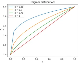
2.5 Unigram distribution . . . 19
2.6 Unigram distribution zoomed up tox=1 . . . 19
2.7 Spearman’s rank correlation results (fastText) . . . 21
2.8 Spearman’s rank correlation results (dict2vec) . . . 22
4.1 Word2vec performance by epoch . . . 34
4.2 Word2vec performance by epoch (boxplot) . . . 34
4.3 Word2vec performance by negative sampling . . . 36
4.4 Word2vec training time by negative sampling . . . 36
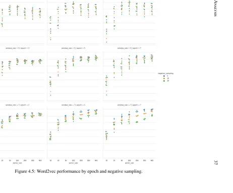
4.5 Word2vec performance by epoch and negative sampling . . . 37
4.6 Word2vec performance by sampling . . . 38
4.7 Word2vec performance by sampling (boxplot) . . . 38
4.8 Word2vec training time by sampling . . . 39
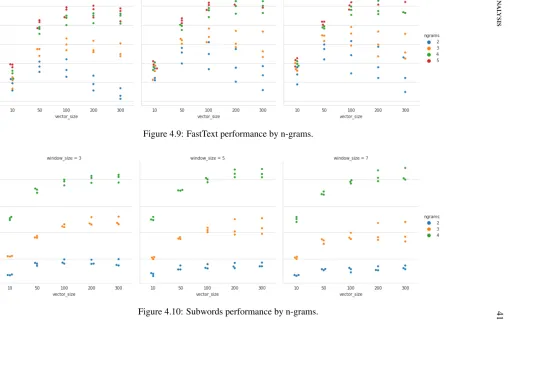
4.9 FastText performance by n-grams . . . 41
4.10 Subwords performance by n-grams . . . 41
4.11 FastText and Subwords performance by epoch and n-grams . . . 42
4.12 Dict2vec performance by epoch . . . 44
4.13 Dict2vec performance by strong draws and beta strong . . . 45
4.14 Dict2vec performance by weak draws and beta weak . . . 46
4.15 Dict2vec performance by strong and weak hyperparameters . . . 48
4.16 DictFastText performance by n-grams . . . 49
4.17 DictFastText performance by strong draws and beta strong . . . 50
4.18 DictFastText performance by weak draws and beta weak . . . 51
4.19 Results for all algorithms . . . 53
4.23 Training time of dict2vec and dictFastText (5-grams) . . . 55
4.24 Spectral clustering on the word analogy task . . . 58
A.1 Term-document matrix . . . 67
A.2 Vector similarity . . . 68
B.1 Monotonic and non-monotonic functions . . . 69
C.1 Details of lexical relations dataset . . . 71
C.2 Laplacian matrix . . . 71
C.3 Normalized Spectral clustering algorithm . . . 72
4.1 Top 5 score results for word2vec. . . 35
4.2 Top 5 score results for fastText and subwords . . . 43
4.3 Top 5 score results for dict2vec . . . 47
4.4 Top 5 score results for dictFastText . . . 47
4.5 Top scores and hyperparameters for each algorithm . . . 56
4.6 Task score breakdown for each algorithm . . . 57
Introduction
Word embeddings are one of the most used representations of vocabulary in NLP. Essentially, a word embedding is a particular mapping of words to vectors (collection of real numbers); addi-tionally, in a confusing way, word embedding is also the collective name of several models that can build said mapping. The possibility to transform words to vectors of real numbers makes them an ideal model to explore and apply several mathematical operations and transformations to hopefully represent some of the features that languages have.
There has been an exploding interest in these kinds of techniques after word2vec [16] was proposed in 2013. A shallow neural network (composed of 2 layers) is used to produce a word embedding, i.e., a vector space where some interesting properties can be observed. One of such properties is vector similarity (in terms of semantics). Given that words are now vectors, several similarity functions can be applied as a quantifiable way of comparing such words. A good word embedding would map similar words to similar vectors, and would map not so similar words to not so similar vectors. For example: the vectors for cat and dogshould be more similar than say, cat and flower. Another property is analogies. This aspect of word embeddings has gained a lot of popularity after word2vec successfully modeled this property via addition and substraction operations on the word vectors:king−man+woman≈queen.
The real power of the word embedding approach is that it is an unsupervised learning model, meaning that it works on unannotated data (and text data is widely available nowadays). The way these models learn these numbers is based on analyzing the contexts between different words and using a prediction approach based on the idea of the Neural Probabilistic Language Model [3] which, in turn, is based on the idea of statistical language models: predict words given a certain sequence of pre-occurring words. For example, given the phrase "read the New York", there are some words (like "Times") that are more likely to occur than others. The idea is that if in the training data there are enough examples of this phrase, then it’s possible to calculate the probability of the next word through the frequency of these word sequences.
There are many models and algorithms that create word embeddings, with different ap-proaches. In the last few years there’s been a resurgence in deep learning with several archi-tectures and hyperparameters being proposed; some of them can even use pre-trained word embeddings from other models as a starting point. Moreover, with of all these different ap-proaches, different numbers are obtained for the embeddings, making it really important to have a solid way of evaluating the different results. However, there’s no one universal stan-dard way of evaluating the word vectors and additionally, there are different properties of the word embeddings that can be evaluated, which makes the evaluation and comparison between models inconsistent across different studies.
1.1
Problem Statement
Adding to the situation of the different evaluation methods, all models are implemented in different programming languages, frameworks, and platforms. While this is natural, given the preferences and capabilities of the different options, the fact that they’re all implemented differently can make some comparisons inaccurate. The main motivation for this thesis is both to try different combinations of hyperparameters and also training the models using the same base language and program; several word embedding models share the same base architecture which makes them ideal to use in this scenario. Additional goals are to confirm the usual recommended values for the hyperparameters and also to be able to measure the improvement of the modules or enhancements of the later models to the baseline in a more accurate way.
1.2
Contributions
First, experiments are run to show how much tuning hyperparameters impacts word relatedness and word similarity tasks for five models based on the same base architecture. Graphs show results for some values of hyperparameters using grid search for individual models, and then all together in the same graph; the best five results of the individual models are shown in tables as well. Finally, for the best result of each model, results of the individual tasks are displayed in a table alongside the average scores.
two models which shows a solid middle ground between these tasks is proposed, albeit with a tradeoffwith the training time.
1.3
Vectors
As previously mentioned, vectors are supposed to represent words (at least in word embed-dings; there are other types of embeddings at sentence-level, paragraph-level, character-level, etc.), but certain issues can occur. For example, things like: polysemy, word senses, and inflec-tions can make it difficult to interpret the mapping from the word to the vector; additionally, the way to learn these vectors is through examples and usage, not by grammar or rules, making them dependent on the quality of the text or type of discourse. On top of that, it’s also im-portant to consider that these embeddings are used in different fields; for example, engineers may use them as inputs for apps or other models, whereas linguists may be more interested in exploring properties related to semantics or other related topics (for more specific details about word embeddings, see Appendix A).
Regarding the size or dimension of the vectors, it’s not quite understood what the dimen-sions mean in the different models; moreover, the number of dimensions is a hyperparameter in most, if not all, with some tasks having better results with some specific numbers. In addition, the same number of dimensions could have different results depending on the training data. This makes it more difficult to understand what the vectors are or represent.
Finally, different tasks have different requirements for "word relatedness"; for example, when dealing withpart-of-speechtagging, two words with the same POS tag should be more related than two words that do not, independent of their individual meanings, whereas in other tasks, there’s no such requirement. In the same vein, tasks like plagiarism detection need finer tuning to define what word or phrases could mean, due to things like paraphrasing.
1.3.1
Syntactic Information
1.3.2
Semantic Information
Semantics refers to the meaning of lexical items, like words or phrases. Word embeddings base their representations on meaning, which isinferredby the usage of the word, according to thedistributional hypothesis "Words used in similar context,tend to have similar meanings". There is one problem though: word senses.
Languages tend to "like" polysemous words. One theory is that it makes languages more efficient (recycling of signs, i.e., words and phrases)1. Independently of the reason, strictly
speaking, all words arepolysemousto one degree or another2(although this is a point of
con-tention among linguists). Some languages are also more open to the use of words to describe certain concepts that are related but not the same thing; in these cases, the word can "bleed" over time in the lexicon and become a new word sense. For example the word "eat", even though as a verb it describes the act of putting, chewing and swallowing food in the mouth, it also means to have a meal, and additionally consuming a lot of something. The degree on which all of this is defined is not easy to determine and, on top of that, there’s the complication of differentiate betweenhomonymyandpolysemy. Word embeddings have some problems with this because the only thing that is used in the vocabulary is the word itself, which depending on the data, could have multiple usages in the context data (which would make the representation too general) or, have some word senses totally absent, which would make the word embedding to not capture those meanings.
Lastly, synonyms and antonyms are an important mention. Synonyms are usually well encoded in word embeddings (given that the basis for learning the word is based on semantic information); however, antonyms are not: They are notexplicitlyused when training so there’s no clear encoding in the embedding itself. Additionally, similaritybetween words is not well defined (conceptually speaking), so it’s not clear what the difference is between words that are not related at all with words that are antonyms.
1.3.3
Analogical Information
Simply stated, an analogy is an inference of a relation between two or more lexical items that can be transferred to the same number of other items. Example: "Annoying like nails on a chalkboard". In NLP, analogies are treated more broadly, i.e., as similarities, for example:
"New York is to the United States as Paris is to France".
There arepair-basedandset-basedmethods3and two types of analogies that are commonly
1http://news.mit.edu/2012/ambiguity-in-language-0119
2http://anglisztika.ektf.hu/new/content/tudomany/ejes/ejesdokumentumok/2011/Kovacs_2011.pdf
used:
• Syntactic Analogy: plurals, verb gerunds, prefixes, suffixes (morphology).
• Semantic Analogy: collective nouns, hypernym, hyponym, meronyms, or simple mean-ing.
1.4
Evaluation
One of the problems with word embeddings is that it’s not fully clear how to quantify the quality of them; considering that there are a lot of tasks where word embeddings are used (for example, part-of-speech tagging, semantic, syntactic, paraphrasing tasks, etc.), to evaluate them is not straightforward. Currently, two popular categories exist [2]:
• Extrinsic Evaluation: Using the vectors as features of a downstream task (outside of the word embedding itself).
• Instrinsic Evaluation: Evaluating the vectors by comparing them to human judgement (innate properties of the vectors or the vector space).
1.4.1
Extrinsic Tasks
Some evaluation tasks [2] include:
• Noun Phrase Chunking: Extracting "compact" noun phrases (not containing other NP-chunks) from a sentence (Bigramsnoun+dependent word. Example4: The yellow dog barked at the cat->(the yellow dog), (the cat).
• Named Entity Recognition: Identify names of organizations, brands, people.
• Sentiment Analysis: Text classification task where a piece of text is marked with a label that reflects level of positive, negative or neutral polarity. Examples: customer reviews, tweets.
• Text classification: Mark a piece of text with a label depending on the content. Examples: tag text by topics (sports, news, film).
• Input for Neural Networks: Using pre-trained word vectors as inputs for other models, for example, using GloVe vectors as a starting point for an LSTM.
1.4.2
Intrinsic Tasks
Some examples of intrinsic tasks [2] are:
• Word semantic similarity: word vectors with similar meanings should be closer than word vectors that are not; the more closer, the more similar the words are.
• Word analogy: as mentioned previously in Section 1.3.3, it’s based on the idea that arith-metic operations over the vectors can model certain relations or concepts by association, e.g.,ais toa∗asbis to ?.
1.4.3
Datasets
Some evaluation tasks and datasets, which will also be used in this thesis are:
• MC-305: 30 pairs with a scale of 0 to 4 (the higher the "similarity of meaning", the higher the number).
• MEN6: 3000 pairs with a score scale from 1-50 of human-assigned similarity judgments.
• MTurk-2877287 pairs and a similarity rating with a scale of 1 to 5.
• Mturk-7718: 771 word pairs with mean relatedness scores. Scores were collected on
Amazon Mechanical Turk, with at least 20 ratings collected for each word pair. Rating consists of a 1-5 scale, where 5 stands for "highly related" and 1 stands for "not related".
• RG-659: 65 pairs with a scale of 0 to 4 (the higher the "similarity of meaning," the higher
the number).
• RW102034 pairs of "rare words" and a similarity rating with a scale of 0 to 10.
• SimLex99911: 999 pairs with a scale of 0 to 10.
5https://aclweb.org/aclwiki/MC-28_Test_Collection_(State_of_the_art)
6https://staff.fnwi.uva.nl/e.bruni/MEN
7http://www.cs.technion.ac.il/~shaulm/papers/pdf/Radinsky-WWW2011.pdf
8http://www2.mta.ac.il/~gideon/mturk771.html
9https://aclweb.org/aclwiki/RG-65_Test_Collection_(State_of_the_art)
10https://nlp.stanford.edu/~lmthang/morphoNLM/
• SimVerb-350012: 3500 verb pairs and a similarity rating on a scale of 0 to 10.
• WordSimilarity-35313: 353 word pairs with similarity score from 0 (totally unrelated words) to 10 (very much related or identical words). The dataset used in the evaluation task is based on a further subdivision14 which has 2 extra subsets:
1. ALL: This is the full 353 pairs set.
2. REL: Goldstandard for measuring relatedness (252 pairs), e.g., clothes-closet 8.0. 3. SIM: Goldstandard for measuring similarity (203 pairs), e.g., clothes-closet 1.9.
• YP-13015130 pairs with similarity rating on a scale of 0 to 4.
1.5
Format of the Thesis
This chapter has introduced the problem, where some background for word information was given, explained the types of evaluation tasks, and finally described the evaluation tasks that will be used in this thesis.
Chapter 2 talks about related works, specifically, how the models work in theory. The base architecture is explained, mentioning the modules that will be relevant for the later models.
Chapter 3 is about the models’ code implementations, where a detailed overview is given, due to the difference between a model’s theory and its implementation. Additionally, the pro-posed approach along with the evaluation process are explained as well.
Results of the experiments are shown in Chapter 4, with several graphs for all the different hyperparameters for all the different models for the average scores. The highest values for the models are shown in a table along with the scores for each task for two averages.
Chapter 5 talks about conclusions over the results and Chapter 6 outlines some potential future work.
12http://people.ds.cam.ac.uk/dsg40/simverb.html
13http://www.cs.technion.ac.il/~gabr/resources/data/wordsim353/wordsim353.html
14http://alfonseca.org/eng/research/wordsim353.html
Related Work
This chapter will be an overview on several word embedding and related embedding models. Detailed descriptions on the word embedding models relevant to this thesis are given on later sections, with special emphasis on word2vec’s skip-gram; this is because all the models that are going to be analyzed are based on this architecture. The first two section are a general overview of word embedding models and some sentence embedding models; the third section describes word2vec, defining the basic concepts and ideas, and describing some optimizations over the initial proposal. Later sections deal with the changes and/or enhancements applied to this base model that fastText and dict2vec propose.
2.1
Word Embedding Models
Although word embedding models have been increasedly cited in the last few years, the concept has been discussed for several years before. The idea of vector spaces representing words were discussed previously in computational linguistics asdistributional semantic models; they were eventually realized after some early models such as Latent Semantic Analysis [7] and Hyperspace Analogous to Language [13] appeared. In particular, LSA was very influential in demonstrating that information from contexts was enough to produce representative word spaces with interesting properties, such as representing semantic similarity for word vectors and relating words that don’t co-occur together. On the other hand, HAL had more success in the field of cognitive science as a model representative of semantic memory [6].
In parallel, neural models such as simple recurrent neural networks eventually started to develop. Once computational power increased and the curse of dimensionality was solved by the Neural Language Model [3], neural word embedding models really started to develop. Starting with word2vec [16], and in conjunction with several libraries and frameworks being developed to treat text data, word embedding models made a big impact in the field. Word2vec
is based on training word pairs taken from contexts found in text corpora and it learns to relate words that occur together. Afterwards, several other models were being proposed as improvements of word2vec. Among them, GloVe [18] focuses on incorporating co-occurrence information from counts instead of training the network using probability, arguing that the order on which words are mentioned is important. Although GloVe has been highly cited, there are some people that have criticized the method of evaluation of GloVe vs word2vec for being "not fair"1.
Other examples of later models include: wang2vec [12], which includes the positional in-formation of the context words to improve the embeddings; sense2vec [24], which proposes adding part-of-speech tags to the words in the training data to improve the vectors and dif-ferentiate word senses; fastText [4], which represents the word vectors as a normalized sum of the word vector plus its n-gram subword vectors, partially solving the problem of out-of-vocabulary words and incorporating syntactic properties; dict2vec [23], that proposes to in-corporate semantic information for the words found in dictionary definitions to fine-tune the vectors.
Later, more complex architectures were developed for neural networks (called deep neural networks, unlike the word2vec model, which is shallow, i.e., 2 layers), with models such as Deep Structured Semantic Model [22], originally designed for information retrieval, that uses a deep network and bag-of-words inputs to learn low-dimensional representations, and CoVe [15] that employs an encoder-decoder architecture with 2-layered LSTMs in conjunction with
attention(a network sub-module to help the encoder part of the network remember long sen-tences). Other models trained as language models like ELMo [19] that learns contextualized words (that is, words as a function of their context) which are also character-based, with 2 biLSTM stacked together, and BERT [8] which gets its word representations from learning bidirectional contexts with thetransformer[26] encoder, are some of the latest state-of-the-art methods to be proposed.
2.2
Sentence Embedding Models
Alternatively, other complex models have been proposed, where, instead of word embeddings, these new models can represent whole sentences and even paragraphs. Notably, doc2vec [11], which is also based on the architectures of word2vec, uses a parameter, adocument id, along with the sentence as an input so the model learns both the sentence and its unique id as a vector. On another note, the Deep Average Network or DAN [10], which consists of two fully-connected layers and a softmax layer, can use pre-trained word embeddings by averaging the
word vectors that make up the input sentence to learn the sentence vector.
Recent developments such as the Universal Sentence Encoder [5], which can use DAN or the transformer as part of its internal architecture, and LaSeR2 [1], which uses bidirectional LSTMs, are based on machine translation and an encoder-decoder architecture to learn the representations; the former learns one language, while the latter is language-agnostic.
On the dictionary side, this model [9] also uses an LSTM but it incorporates dictionary definitions to map the word to its definition. By also using pre-trained word embeddings, the authors also built a reverse dictionary, where the input is a phrase or description, and the output is a word; this way, the model learns the definition of the word by making its representation closer to its word vector representation.
2.3
Word2vec
Word2vec [16], consists of a predictive model applied to text data, specifically, co-occurrence data within a sliding symmetric context window; this window is made from the middle word (called thetarget word) and its surrounding words (context words):
Example: "The snow is white"
Context 1:
• Target word: snow
• Context words:The,is
Context 2:
• Target word: is
• Context words:snow,white
The main idea is to feed the model different contexts and learn which words co-occur in the same context; in other words, it aims to find good representations of words that can predict other words that occur in similar contexts. This is fairly similar to Probabilistic Language Models, where given a sequence of words, the next word is predicted. The main problems with these kinds of models are the "Curse of Dimensionality" (where the number of variables for the sequences explodes as the vocabulary grows) and that once the model is trained, it’s not possible to calculate the probability over a previously not seen sequence (because there’s no training data, it’s impossible to calculate the probability over counts).
2Although this is the name of the released framework, the reference is the study where its learning architecture
Both of these problems were minimized by the Neural Probabilistic Language Model [3] through the use of a shallow neural network; because this model doesn’t use the frequency of words (it tries to fit the known data with neuron weights and it tries to generalize from that). Word2vec uses a similar architecture and the same base idea.
Word2vec has 2 different "versions" of training:
• Continuous Bag-of-Words: Predicts a target word given the context words.
• Skip-Gram: Given a target word, predicts the context words.
For both of these cases, the model tries to maximize the log probability of the output word(s) given the input word(s). That means predicting through probability the context words given the target word in the case of Skip-Gram and the target word given a context word in the case of Continuous Bag-of-Words.
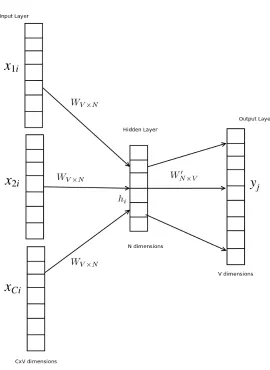
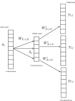
Figure 2.1 shows the architecture of CBOW. Note thatV is the size of the vocabulary (the number of words that are going to be trained in the model). Words xci represent the context
words in one-hot encoding; this means that the currenti-th value (which is the position of the word in the vocabulary) of the input vector is 1, and 0 for all other values. hi is the vector
representation of word xci, C the size of the context, and j the position of the target word in
the vocabulary. Skip-Gram, depicted in figure 2.2, follows the same notation as CBOW, with the difference that now the input (xi) is the target word and the outputsyc j will be the context
words.
One important variable is the dimension of the vectors (which isNand is a hyperparameter of the model); while the model is originally trained for finding good representation of words that can predict co-occurring words, the ultimate objective is to learn low-dimensional repre-sentations of the words in the vocabulary (which are originally represented with dimensionV, the size of the vocabulary). Notice that because the model has words in both its input(s) and output(s), the dimensions of the weight matrices are inverted in order to match the multiplica-tion of the vectors.
Cost function (Continuous Bag-of-Words Model):
J= max(
C
X
t=1 n
X
k=−n
logp(wt|wt+k)) (2.1) p(wt|wt+k)=
evt·vt+k
P
w∈V
Figure 2.2: Skip-gram model; input is thetarget word, outputs areC context words. And for Skip-Gram:
J= max(
C
X
t=1 n
X
k=−n
logp(wt+k|wt)) (2.3) p(wt+k|wt)=
evt+k·vt
P
w∈V
ev·vt (2.4)
where, for both cases, w is a word in the vocabulary, wt is the target word, wt+k a context
word, vis the vector for word w, and vi is the vector for wordwi. For CBOW, context word
vectors are taken from their corresponding rows ofWand the target word vector is taken from its corresponding column ofW0; conversely, for skip-gram, the target word vector is taken its corresponding row ofW and context word vectors from their corresponding columns ofW0.
In both models, the input layer is also calledthe embedding layer, the second layer is called
finished training, the hidden and output layers are removed. This causes the output to now be the low-dimensional vector representation of the input word (this process is common in learning models, where the goal is to train the model for a certain task and the objective is to get a good representation instead of the predictive model itself3).
Additionally, while the embeddings of both architectures are comparable, according to Mikolov4 that skip-gram needs more data and represents infrequent words well; conversely,
CBOW is faster to train and it represents frequent words slightly better. This is probably because for CBOW, more input data points with the same output are generated5.
2.3.1
Skip-Gram
In this section, Skip-gram will be explained over CBOW because the other models analyzed are based on this architecture; for more in-depth analysis of the formulas specifically to word2vec, read this document6).
Vocabulary and Weights
The architecture, as previously stated, consists of 2 layers of neuron weights plus an output layer. The number of weights in each layers is the same as words in the vocabulary (so every word has a set of weights), meaning that some pre-processing must be made beforehand to determine the vocabulary. Because too rare words are not useful (because they don’t appear in enough contexts) a cut-offfrequency is commonly used where words below a certain frequency are deleted (or ignored) from the input data.
Embedding
A training input will be a word pair (target word-context word) obtained from a context; a context is obtained by moving a sliding window over the text. The context size (how many words from a context), from now on called window size, is a hyperparameter. Because the data is read as this moving window, all punctuation is removed and all text is put in one line (separated by spaces) so the sliding window can move through all words, not taken the structure of text into account (titles, paragraphs, etc.).
For example, given the following sentence, with a window size of 5 (some sources use the number of context words at either side of the target word; in this work, the word2vec
3http://mccormickml.com/2016/04/19/word2vec-tutorial-the-skip-gram-model/
4https://groups.google.com/forum/#!searchin/word2vec-toolkit/c-bow/word2vec-toolkit/NLvYXU99cAM/
E5ld8LcDxlAJ
5https://groups.google.com/forum/#!msg/word2vec-toolkit/LNPeC5gyhmQ/p8683JkD6LoJ
convention is used, which is all words in the window) "The waves were crashing on the shore", generates the folowing target word, context word pairs (edges ignored):
• "the waves were crashing on":(were, the), (were, waves), (were, crashing), (were, on)
• "waves were crashing on the": (crashing, waves), (crashing, were), (crashing, on), (crashing, the)
• "were crashing on the shore": (on, were), (on, crashing), (on, the), (on, shore)
Now, given that the neural network weights can be modeled as a matrix (one for each layer), with each row of the matrix corresponding to each word in the vocabulary and the input is a vector (using one-hot encoding), then the embeddinghifor input wordwi (the target word) can
be defined as:
hi = w T
i · xi (2.5)
wherexiis thei-thword in the vocabulary. Because this input is in one-hot encoding, then this
is the same as just taking thei-throw of weight matrix W. This works for both layers of the model.
Error Function
The objective function is the log probability of the context wordwcgiven the target wordwt:
−logp(wc|wt) (2.6)
In other words, the desire is to maximize the probability of the model outputting the context word given the target word. Because several contexts exist, then given a target there’s going to be a big range of likely words and these probabilities are adjusted (or learned) by modifying the weights. According to this angle, this is really similar to a multi-classification problem (having the output wordswc as the classes), and given that the outputs are probabilities, then
softmax (Section 2.3.1) is suitable.
Output
softmax function, and then changing the weights of the two previous layers via back propaga-tion (Secpropaga-tion 2.3.1).
F(xi)= exi
k
P
j=1 exj
(2.7)
Updating Weights
After making a prediction in a training pair, the error is calculated and the weights are modified according to the product of the error and the gradient of the output of said layer. The idea is to apply gradient descent to find the optimum weight value which would minimize the error of both sets of weights.
After modifying the weights of the hidden layer, then the same process is made for the previous layer but instead taking the gradient of the activation function of the next layer. Be-cause each gradient depends on the output of the layer, this process is called back propagation because the errorspropagatethrough each layer (to put it differently, the output of a layer de-pends on the output of the previous layer). For more details on how to calculate the gradients, see [20].
2.3.2
Optimizations
In a follow-up paper [17], the authors mention several implementation details to speed up the training process. The most important (and cited) are:
• Hierarchical Softmax
• Negative sampling
Hierarchical Softmax
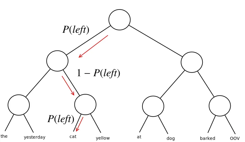
Because calculating the softmax denominator output is expensive (going throughallwords in the vocabulary), a binary tree can be built with the leaves of the tree being the words in the vocabulary. Then, the probability of a word is given by the path from the root to the leaf node. This way, it is only necessary to evaluate log2(vocab_size) at most.
one.
Sigmoid can be used as a function to get probabilities at each node, which is defined as the similarity between the representation of the word and a coefficient vector7 which can be defined and learned in a multitude of ways; they can be seen as weights of the hidden layer in the neural network model.
P(left)=σ(v0Tnvw) (2.8)
P(right)=1−P(left) (2.9)
withv0Tnbeing the coefficient vector for noden.
Example: "The yellow dog barked at the cat".
Figure 2.3: Hierarchical Softmax
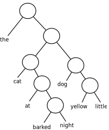
Also, the way in which the tree is built, impacts the performance directly. The authors also proposed to use Huffman encoding so that more common words are closer to the root, further improving performance.
Figure 2.4: Huffman encoding; words that are more common will be closer to the root.
Negative Sampling
An alternative to softmax (based on Noise Contrastive Estimation, or NCE). Given that the model is only interested in learning high-quality vector representations, the objective function can be changed to use pairs of words, instead of a probability distribution. In a simplified way, only "good pairs of words" (or good examples) are needed to train the model; in this vein, it can be argued that "negative examples" make the algorithm learn a generalized representation and "positive examples" make the algorithm learn a specific representation. These negative samples are sampled randomly from the vocabulary given a noise distribution. A good distribution, according to the authors, is the unigram ditribution:
U(w)α
n
P
i=1
U(wi)α
(2.10) Figures 2.5 and 2.6 show how this distribution looks for different values ofα; the authors mentioned that α = 34 gave the best results for the model. It was also suggested that a good number of negative samples is between 5-20 for small datasets and 2-5 for large datasets.
Figure 2.5: Unigram distribution
J = −
|C|
X
i=1
L log(σ(wt·wci))− K
X
k=1
(1−L) log(1−σ(wt·wnk))
!
(2.11) withKbeing the number of words sampled from the noise distribution (and a hyperparameter),
Lthe label of the word pair,S the sigmoid function: S(x)= 1
1+e−x,wtthe vector for the target
word taken from the embedding layer weightsW,wcithe context wordifrom the hidden layer
weightsW0, andwnkthe wordkfrom the noise distribution (the negative sample).
The resulting training process is now changed to a positive sampling operation plus K
negative sampling operationsfor each target word and context word pair.
2.4
FastText
Proposed in [4], it uses the same architecture as skip-gram of word2vec, but makes a small but important change. Instead of just using words in the vocabulary, subword character n-grams are also learnt; a word representation is now the normalized sum between the representation of its subwords and the whole word. This means that for a word likeapple, the generated tokens will be: <ap, app, ppl, ple, le>, apple(having <and> as the start and end delimiters for the word, respectively). This also slightly increases the vocabulary size and a function has to be used to find the subword n-grams or they can be pre-computed.
The objective function is updated to maximize the summation of the representations:
J = C
X
t=1 n
X
k=−n
X
w∈Gwt
logp(wt+k|w) (2.12)
One strength about fastText in contrast to word2vec, is that these word vectors give the possibility of representing out of vocabulary words (OOV) by just using their subword vectors. Figure 2.7 shows results of evaluating8the word vectors on several tasks of word similarity
and word relatedness in languages such as: Arabic (AR), German (DE), English (EN), Spanish (ES), French (FR), Romanian (RO), and Russian (RU). The two english tasks are also evaluated in this thesis and are described on Section 1.4.3.
8The score is the Spearman’s rank correlation coefficient between human judgement and cosine similarity over
Figure 2.7: Spearman’s rank correlation between human judgement and cosine similarity of fastText vectors for different tasks in different languages (results are multiplied by 100). Columns sg and cbow are both of word2vec’s implementations; sisg- is the Subword Infor-mation Skip Gram (fastText) when representing OOV words asnull and sisg when subword vectors are used to model OOV words. The languages evaluated are: Arabic (AR), German (DE), English (EN), Spanish (ES), French (FR), Romanian (RO), and Russian (RU) (image taken from source paper [4]).
2.5
Dict2vec
Dict2vec [23] also uses the same architecture as skip-gram but tries to add semantic information from word definitions to the training process. Additional sampling steps are added: sampling new words from sets defined as eitherstrongorweakdepending on their mutual appearance on dictionary definitions (which are taken from different dictionaries online). For example: if the wordroadappears in the definition ofcar, and viceversa, then they form astrong pair; if only one of the words appear in the other’s definition, then they form a weak pair. Additionally, pre-trained word embeddings can be used to help define if words can be astrongorweakpair depending if they mutually appear in their k-nearest neighbors. Additionally, this model also uses negative sampling and the same weight initialization as word2vec.
The objective function is changed to this:
J(wt,wc)=`(vt·vc)+Jpos(wt)+Jneg(wt) (2.13)
Jpos(wt)=βs
X
wi∈Vs(wt)
`(vt·vi)+βw
X
wj∈Vw(wt)
`(vt·vj) (2.14) Jneg(wt)=
X
wi∈F(wt)
wi<S(wt)
wi<W(wt)
`(−vt·vi) (2.15)
One additional constraint is that the negative samples can’t belong to the strong or weak sets of the target word, as shown in equation 2.15.
According to the authors, this model gets better results than word2vec and fastText for both word similarity and text classification evaluations and it’s also claimed that it has less training time (it takes less time to reach the optimum); however, it uses more hyperparameters (the
strongandweaksampling and beta values (for the strong and weak sampling).
Table 2.8 shows the published results of evaluating several word similarity tasks on the dict2vec embeddings using the Spearman’s rank correlation coefficient (scores are multiplied by 1000); this method of evaluation is going to be reutilized for this thesis, hoping to replicate results.
Figure 2.8: Spearman’s rank correlation coefficient (scores multiplied by 1000) between human judgement and cosine similarity of word vectors (top) and accuracies on text classification tasks (bottom). Models analyzed are word2vec, fastText, and dict2vec (labelled asours). Corpus A is Wikipedia, whereas corpus B is Wikipedia + the dictionary definitions concatenated; the 50M & 200M refer to the first 50 million and the first 200 million words from Wikipedia, respectively (image taken from source paper [23]).
Model Implementations and Evaluation
In this chapter, technical and specific details about the implementations are discussed. Given that the theory of how the models work differs slightly from the actual implementations (mostly due to inherent limitations of the medium, such as hardware or memory), special attention is given to these aspects of the models, which are sometimes not covered. As mentioned in previous chapters, given that both fastText and dict2vec are based on skip-gram, only this model will be discussed; this chapter also presents this thesis’ main contribution: a hybrid model of fastText and dict2vec.
In addition, the method of evaluation of the models is presented along with descriptions of the experiments such as: training data and preprocessing, hyperparameter discussion, and details about extra information needed for both dict2vec and the proposed model.
3.1
Word2vec - Skip Gram
The code is written in C and it’s available on GitHub1. It is important to note that all the mul-tiplication routines are done in basic C with no external libraries; it’s also highly optimized for several other tasks such as random values, shuffling and the activation function. The repository also contains other programs related to word2vec and scripts with demos and basic evaluation tasks.
In terms of how it works, the program reads the input, which is a text file of words written in a single line separated by spaces, builds the vocabulary and creates the sampling table. The sampling table is a big array of 10 million values where each value in the array is going to be the index of a word. The amount of times each value appears in the table is given by:
1https://github.com/tmikolov/word2vec
frequency= f 3 4
PV
i=1 f 3 4
i
×ts (3.1) with fi being the sum of all counts to the 0.75 power andtsis the size of the table (107).
After the sampling table is filled with values, it gets shuffled so the same values are not contiguous. Then, the input file is divided into chunks which are then given to a set of threads that go through every word (a thread per chunk). For every word, the context window is calculated (edges are ignored) and for each pair of target and context words, negative words are sampled from the sampling table. Because of the sampling table shuffling, an index at the start of the array that goes through it is enough to simulate the random sampling.
An additional hyperparameter calledsamplingis used: it is used to calculate the probability of discarding a word when going through the input. The probability of discarding the word is defined as:
p(w)= 1−
r
t
f(w), where t is the treshold (the sampling hyperparameter) and f(w) is the proportion of the wordwin the corpus, i.e., f(w)= count(w)
N , where N is the total number of
words. The intention of this is to train the model with words that are not so frequent because words that are too frequent tend to have no meaning (stopwords). The usual recommended value for sampling is 0.0001.
After the positive and negative samples are obtained (1 positive + n negatives), logistic regression is applied to the dot product of the vectors, where the error is obtained. That value gets multiplied by the learning rate to obtain the gradient, which will be used to modify the weights of both layers. Through backpropagation, the output weights get updated first by the gradient multiplied by the input word vector, and then the input weights are modified after all samples are processed by the accumulated sum (of all samples) of the gradient multiplied by the output word vector.
After the epochs have finalized, then the program goes through every word in the vocab-ulary and writes a .vec file with the vector representation of every word (one for each line, where first comes the word and the weight values, all separated by space). Notably, this imple-mentation also has the option of using either hierarchical softmax or negative sampling for the training.
3.2
FastText
cal-culates the subwords and adds them to asubword vocabularywith their own weights and the list of indices of the subwords are stored in the structure of the word. Then, at training, when reading a word, the program gets the weights of the subwords (via the list of indices) and adds them. Afterwards, the vector of the full word is added to this sum and then it’s averaged. Note that this sum is only calculated for context words (the input weights). The rest remains the same.
The process of updating the weights is mostly the same, the only change is that each of the subwords weights are also going to be modified by the same amount as the input weights. This implementation also gives the option to choose between hierarchical softmax and negative sampling. The original code2is in C++, although there’s a fairly popular python implementa-tion in gensim3. It’s also important to mention that the published program also allows one to use the word embedding for text classification problems.
3.3
Dict2vec
This code is a re-implementation of the skip-gram base code, it’s also written in C and it doesn’t have hierarchical softmax available. The big change is the additional sampling of the dictionary words, from both the strong and weak sets; basically two extra steps after updating the output weights (the normal positive and negative sampling) but before updating the input weights (because this uses the sum of all the output words multiplied by the gradient). In this model, the number of words sampled from each set as well as the beta (learning rate) of each sampling are hyperparameters.
The process itself is a form of positive sampling but from semantically related sets. The idea is that when training the context word, it’s possible to randomly sample the set of definition-related words (both the strong and weak sets) to add semantic information (just like negative sampling, but in this case the label is positive). In other words, normal positive sampling finds word pairs that co-occur in a given context in writing, and dict2vec positive sampling finds word pairs that co-appear in word definitions.
3.4
Proposed Model (dictFastText)
The implementation of this proposed model is based on the Dict2vec C code with the subword embedding process added, and was dubbeddictFastText. This means that training is the same as it is in fastText (with a word being the normalized sum of the internal subwords that make
2https://github.com/facebookresearch/fastText
the word), but after the positive and negative sampling training is done for a word pair, then the strong and weak sampling from dictionary word pairs is applied.
To sum up, for a given word pair (wi,wj), the process is as follows:
• build the word embedding swi with subwords of the target word wi and apply logistic
regression over this positive sample.
• sample negative pairs of the context wordwj (word2vec negative sampling) and apply
logistic regression.
• sample pairs from the strong set of words forwjand apply logistic regression.
• sample pairs from the weak set of words forwjand apply logistic regression.
The hypothesis is that this hybrid model can have some of the syntactic properties and the capability of representing words not in the vocabulary of fastText and the high performance over word similarities demonstrated by dict2vec.
3.5
Evaluation
3.5.1
Experiments
Word Semantic Similarity
This task is a replication of the process of evaluation applied in dict2vec [23]. It consists of comparing the tasks’ evaluation scores (described in Section 1.4.3) against a similarity metric score applied on the embeddings. The chosen similarity metric was cosine similarity (same as the dict2vec evaluation process):
similarity= cos(θ)= A·B
||A|| · ||B|| =
n
P
i=1 Ai·Bi
rn P
i=1 A2
i
rn P
i=1 B2
i
Said average score is the micro average, which is calculated by:
PT
i=1Si·Ni
PT i=1Ni
(3.3) whereT is the number of tasks, Si the score (the Spearman’s rank correlation coefficient) of
taski, andNi the number of samples (word pairs) in taski.
The reason to use this metric was not backed by the authors, but it’s usually employed when there’s a significant difference in the number of samples of each task; this is because the score of each task is proportional to its number of samples. In this case, the lowest number of samples is 30 while the maximum is 3500, so it’s highly likely that this was the reason to do so. On top of this, because each task has a different focus (for example, a task contains only verbs, another one only rare words) it can happen that the score can be skewed to certain tasks. To give a better view of performance, a macro average (the average of the task scores) was added to show how the models perform across all tasks.
Additionally, training time is also analyzed for this task, with lower being better and mea-sured in minutes. Lastly, as a note, the evaluation script was slightly modified to add support for the models with n-grams.
Word analogy
As previously mentioned, the word analogy property can be generalized to pairs of words that display some kindof relation. Based on this view, Diffvec [27] is a dataset built to evaluate several lexical relations that can be represented by vector differences (see Appendix C for more information). Essentially, there are 9 classes such as:collective noun,hypernym,meronym, and
singular-pluralthat represent said relation between words; the idea is to evaluate if the word embedding can produce vectors that show these relations through vector differences (Section 1.3.3).
embeddings, they’re an abstract concept.
3.5.2
Training Data
The same corpus of dict2vec is used (Wikipedia dump from July 20174), however, due to time
constraints and the number of hyperparameters, only the first file (the first 50 million words) is going to be used for training.
The preprocessing is the same as the one applied by dict2vec5 which is quite simple: all text is lowercased, and only characters in the english alphabet are kept, except digits which are translated to words, e.g., 1 turns toone. All text is then written in one line with words separated by space.
3.5.3
Web Scraping
To obtain the strong and weak pairs data, the words from the vocabulary (which is made from all words with a frequency of 5 and more) are searched in these oline dictionaries: Cambridge6, Collins7, Dictionary.com, and Oxford8; all pages were downloaded and only the HTML
ele-ment with the definitions’ texts were saved to disk. This method was preferred because if there’s any IP blocking or disconnect midway, the files are saved.
Because the way to access these webpages is by a direct URL, some websites return a 404 response and those webpages can be ignored; however, there’s other websites where accessing a non-existing URL triggers a search page, so the only way to check if the dictionary has the definitions for the word is to actually analyze the webpage. The base program was modified to read these files from disk instead of downloading them. An additional script was made to delete files with no definitions.
3.5.4
Hyperparameters
As mentioned before, one objective is to reproduce and confirm the usual recommended values for hyperparameters of the models. After the values were selected, the models were then trained using grid search over seven epochs and word embeddings were saved for the third, fifth, and seventh epoch. Experiments were run with 8 threads each, on a linux machine with its CPU being an Intel i7-7700K @ 4.20GHz.
4Obtained from https://dumps.wikimedia.org/enwiki/, although the used corpus is no longer available.
5Although the perl script to preprocess the data is available in the dict2vec’s github page, the original can be
found here http://www.mattmahoney.net/dc/textdata.html
6https://dictionary.cambridge.org/dictionary/english/
7https://www.collinsdictionary.com/dictionary/english
The hyperparameters are:
• Vector size: Size of the vectors. Usual recommended values are 100 and 300.
• Window size: Number of words in each context. Usual recommended value is 5.
• Sampling: Threshold factor to estimate the probability of discarding a word (as described in Section 3.1). Usual recommended value is 0.0001.
• Negative sampling: Number of words sampled from the noise distribution (described in Section 2.3.2). Usual recommended values are 2-5 for big datasets and 5-20 for small datasets.
• Ngrams: size of the subwords (described in Section 2.4). Recommended values are 5 and 6.
• Strong draws: Number of words sampled from the strong set (described in Section 2.5). Recommended values are 2-5.
• Beta strong: Factor that multiplies the positive strong sampling (described in Section 2.5). Recommended value are 0.5-1.2.
• Weak draws: Number of words sampled from the weak set (described in Section 2.5). Recommended values are 2-5.
• Beta weak: Factor that multiplies the positive weak sampling (described in Section 2.5). Recommended values are 0.2-0.6.
The selected hyperparameters for word2vec were:
• Vector size: 10, 25, 50, 100, 200, 300, and 400.
• Window size: 3, 5, and 7.
• Sampling: 0.1, 0.01, 0.001, and 0.0001.
• Negative sampling: 5, 10, and 20.
For FastText the hyperparameters chosen were:
• Vector size: 10, 50, 100, 200, 300.
• Sampling: 0.0001.
• Negative sampling: 5.
• Ngrams: 2, 3, 4, and 5.
For dict2vec the hyperparameters chosen were:
• Vector size: 10, 50, 100, 200, 300.
• Window size: 3, 5, and 7.
• Sampling: 0.0001.
• Negative sampling: 5.
• Strong draws: 2, 4, and 8.
• Beta strong: 0.2, 0.4, and 0.8.
• Weak draws: 2, 5, and 8.
• Beta weak: 0.3, 0.45, and 0.9.
For dictFastText, the hyperparameters chosen were:
• Vector size: 100, 200, and 300.
• Window size: 3, 5, and 7.
• Sampling: 0.0001.
• Negative sampling: 5.
• Strong draws: 4 and 8.
• Beta strong: 0.4 and 0.8.
• Weak draws: 5 and 8.
• Beta weak: 0.45 and 0.9.
Results
This chapter shows and discusses the results over the experiments defined in the previous chap-ter, with the first section dealing with the hyperparameter tuning for each model individually. In general, all results are shown in graphs for each model for qualitative results, and tables for quantitative ones. The reader should note how the different combination of hyperparameter values affect the models; for this effect, some additional type of graphs (such as box plots) are shown to try to highlight different views of the results. Towards the end of the section, results of all models are shown in the same graph to have a better idea how they compare to each other. At the end of the chapter, the highest performances are selected for each model and shown in a summary table including the performance over each task. On top of this, a less-known additional evaluation is applied to the models to evaluate a different aspect of the embeddings and show that it appears there’s some indirect relationship between the two properties.
4.1
Analysis
It’s important to remember that some hyperparameters of the models were mantained constant in all experiments such as the learning rate (locked at 0.025) and the cutofffrequency of words for the vocabulary (5, meaning that words with frequency of 4 and less were ignored). Also, as mentioned before, the micro average of the Spearman’s rank correlation coefficient is going to be considered as the metric for evaluation and, to a small extent, the training time as well. Each experiment was run once, saving the vectors for epochs 3, 5, and 7; that means that one experiment appears three times on any given graph (unless plotting separate epochs).
Regarding the graphs, given the high number of experiments in some of the models and that hyperparameter values are discrete, swarmplots were preferred; swarmplots, in essence, work just as scatterplots. The main difference is that swarmplots try to show or display more data points when there are many of them by exploiting the horizontal space (which is possible
because of the discrete values in the x-axis), whereas in scatterplots, those data points would not be visible because most of them would be superimposed, making it harder to analyze the results. Boxplots were also added to this end, hoping that information from both types of graphs can give a good view of the results.
4.1.1
Word2vec
As a note, the plotting of the sampling hyperparameter was changed to its exponential value to make it easier to graph results; also, time values in plots are in minutes.
C
hapter
4.
R
esul
ts
Figure 4.1: Word2vec performance by epoch, note how higher results are associated to higher epochs.
Figure 4.3 shows that for window sizes 5 and 7, lower negative sampling values tend to have higher results (for window size 3 it’s similar but it seems to be less clear). This also confirms that the usual recommended value for negative sampling (5); apparently it seems that trying to learn too much from negative examples disrupts the learning from the positive sampling. It can be seen in Figure 4.4 how adding more samples also makes it much slower. Finally, Figure 4.5 shows results divided by epoch and window size in order to see them more granularly.
Figures 4.6 and 4.7 show some interesting results: the usual recommended value of 0.0001 (or -4 in the log scale) has consistent high scores for windows sizes 3 and 5 for vector sizes 100 and lower (for greater values -4 and -3 are on par). With window size 7 there’s a less clear scenario in the higher scores with a mix between all values for the hyperparameter; looking at the box plot, it seems that -3 seemes to have a higher max and median, although the difference looks minimal. Window size 7 seems to have better results than other windows, specially at higher values of vector size; this seems to indicate that the decision of window size could be more important than the sampling value.
Regarding training time, Figure 4.8 shows how increasing the sampling hyperparameter af-fects its training time; increasing the value means training more words because the probability of discarding a word is lower. It’s important to note that although increasing this hyperparam-eter makes the model to havesomewhatbetter results, the training time is considerable higher; hence, a sampling of 0.0001 is good enough because the performance increase is negligible.
epoch vector size window size sampling negative sampling average score time 7 400 7 -2 5 0.450 14.295 7 400 7 -3 5 0.450 11.349 7 300 7 -3 5 0.449 9.468 7 400 7 -4 5 0.446 8.110 7 300 7 -2 5 0.445 11.964
C
hapter
4.
R
esul
ts
Figure 4.3: Word2vec performance by negative sampling.
A
n
al
ysis
37
C
hapter
4.
R
esul
ts
Figure 4.6: Word2vec performance by sampling.
A
n
al
ysis
39
4.1.2
FastText
For fastText, some interesting results were obtained. Figure 4.9 shows how increasing the number of n-grams raises performance; this makes sense because 4-grams and 5-grams are getting closer to actual words. It was surprising to see that 3-grams had very low scores, because one good strength about 3-grams is that it’s possible to reconstruct (almost) all words. Additionally, extra experiments were defined to check the performance of fastText using only subword n-grams and skipping the addition of the whole word; this implementation was namedsubwords. Figure 4.10 shows the subwords embeddings; results are somewhat similar to fastText and also shows better performance as n-grams increase. One key difference between fastText and subwords is that words shorter than ngram_length − 2 can’t be represented in
subwords1. This can be important if shorter words are needed and it’s obviously dependant on n-gram length, with only being a significant problem for n-grams greater than 4. There are some possible solutions to this: for example, using the whole word only in these cases, or adjust the number of n-grams on the fly depending on the length of the word; in this work however, these options were not tried.
Figure 4.11 shows both variants in the same grid for different epochs. Surprisingly, it seems that adding the word doesn’t have that much impact in the embeddings, although maybe this doesn’t occur when using more training data, bigger vector sizes, or bigger window sizes. In any case, if this holds, then smaller embedding files can be used without too much of a loss in performance.
1For example, given 5-grams, the worddogcan be represented by:’<dog>’; on the contrary, a word like’do’
has the following n-gram: ’<do>’, which is shorter than a 5 gram and thus, can’t be represented. In the case of
A
n
al
ysis
41
Figure 4.9: FastText performance by n-grams.
C
hapter
4.
R
esul
ts
algorithm epoch vector size window size n-grams average score time ft 7 300 7 5 0.492 17.731 ft 5 300 7 5 0.482 17.731 ft 7 200 7 5 0.482 13.161 ft 7 300 5 5 0.479 12.786 ft 7 200 5 5 0.479 9.514 sw 7 300 7 4 0.444 11.336 sw 7 300 5 4 0.440 7.821 sw 7 200 5 4 0.438 5.831 sw 7 200 7 4 0.435 8.429 sw 5 200 5 4 0.422 5.831 Table 4.2: Top 5 score results for fastText (top 5) and fastText with no word added (bottom 5). Time is measured in minutes.
4.1.3
Dict2vec
Figures 4.12 and 4.13 show some interesting results: almost all top scores have values of 4 and 8 for the strong draws and 0.4 and 0.8 for the beta strong; conversely, 2 strong draws are almost at the bottom with a handful at the top. This implies that higher values of the strong set variables have an important role in higher score values. This is slightly different from the results proposed by the authors where 4 strong draws and strong beta 0.4 were mentioned as the optimum; however, the authors did give some intervals where all these variables would be better, so it could depend on the dataset.
C
hapter
4.
R
esul
ts
Figure 4.13: Dict2vec performance by strong set draws (left) and beta of strong set sampling (right)