On the Use of Financial Data as a Random Beacon
∗Jeremy Clark
University of Waterloo
Urs Hengartner
University of Waterloo
Abstract
In standard voting procedures, random audits are one method for increasing election integrity. In the case of cryptographic (or end-to-end) election verification, random challenges are of-ten used to establish that the tally was computed correctly. In both cases, a source of randomness is required. In two recent binding cryptographic elections, this randomness was drawn from stock market data. This approach allows anyone with ac-cess to financial data to verify the challenges were generated correctly and, assuming market fluctuations are unpredictable to some degree, the challenges were generated at the correct time. However the degree to which these fluctuations are un-predictable is not known to be sufficient for generating a fair and unpredictable challenge. In this paper, we use tools from computational finance to provide an estimate of the amount of entropy in the closing price of a stock. We estimate that for each of the 30 stocks in the Dow Jones industrial average, the entropy is between 6 and 9 bits per trading day. We then pro-pose a straight-forward protocol for regularly publishing veri-fiable 128-bit random seeds with entropy harvested over time from stock prices. These “beacons” can be used as challenges directly, or as a seed to a deterministic pseudorandom generator for creating larger challenges.
1
Introductory Remarks
In many countries, including the United States, tronic elections have become predominant. Some elec-tronic voting technologies additionally provide a paper-based record of each vote—e.g.,optical scan and DRE machines with voter-verified paper audit trails. This pa-per record can be compared with the electronic tally, and while both tallies could be consistently manipulated, this check does provide some level of assurance that the elec-tronic tally is correct. It is not feasible to perform this
∗Full version.Contains some corrections and revisions to the ver-sion that appeared at EVT/WOTE 2010.
check for all precincts; however by randomly selecting a small number of precincts in an unpredictable way, ex-cellent statistical assurance of the consistency of these tallies can be achieved.
This mathematical approach to protecting against er-rors and manipulation in elections can be taken a step further. Cryptographic voting systems use mathematical techniques throughout the entire voting process to pro-vide a stronger notion of integrity: even if all the records of all the ballots are subverted, the manipulation will be reliably detected. In many cryptographic systems, assur-ance is established by challenging the system to prove computations were performed correctly. As with choos-ing precincts, challenges in cryptographic votchoos-ing must be random.
This paper is concerned with choosing a source of ran-domness to generate these random selections or chal-lenges. We will speak abstractly and phrase the nature of the random action as selectingunitstoaudit (follow-ing [36]). It is hopefully intuitive that if the source of randomness used to select units is predictable or can be influenced, the statistical assurance loses strength.
One proposal for an unpredictable source of random-ness is financial data (we review a number of other pro-posed methods in the next section). While not broadly adopted, this technique has been used in at least two binding cryptographic elections: a university election with Punchscan [21] and a municipal election with Scantegrity II [11]. In both cases, cryptographic tools were used to transform the random financial data into a useful form. This may lead some to object to using this type of protocol in non-cryptographic voting contexts, like precinct selection. Our position here is neutral—its application to cryptographic voting is motivation enough for this study, and we note that if cryptographic tech-niques were permissible for use, then this approach does provide a more publicly verifiable challenge than, say, rolling dice in a room.
like stock market prices, exhibits some unpredictable be-haviour, but it is not likely intuitive how much random-ness there is. In this paper, we combine a model from computational finance with techniques from information theory to estimate the amount of entropy in the daily closing prices of a number of common stocks (the same set used in the Scantegrity II election). In our sample, a typical closing price has an estimated 6–9 bits of entropy. When we consider the joint entropy between two highly correlated stocks, we find that the joint information is less than a single bit, suggesting that using a portfolio of stocks is a good method of increasing the pool of entropy. Finally, we present a straight-forward protocol that can be used to take the prices in their raw form and produce a near-uniform random bit string. Our intention is that some entity will publish the output from our protocol on each day that the market closes as a service. As an in-centive to offering this service, we allow the entity to mix in their own randomness. This is done in a way that is transparent and verifiable to everyone to ensure that the entity will be caught if it misbehaves. The output can then be used either directly to select units for auditing, or if many bits are required, the output can be used to seed to a pseudorandom generator. The output is also useful for non-voting cryptographic protocols where a beacon or common reference string is required.
Contributions. In this paper, we present the following:
• a general technique for estimating the amount of entropy in a stock market closing price that is ex-tensible to any simulatable model in computational finance,
• a set of empirical estimates of the entropy in a repre-sentative portfolio of stocks, under the conservative assumption that the Black-Scholes model holds for market behaviour,
• a demonstration of the impact on entropy that the four parameters—drift, diffusion, initial price, and time period—have within the range of our data, • an estimate of the mutual information shared by
cor-related stocks within the same business sector, and • a protocol for regularly publishing verifiable
ran-dom bitstrings based on stock prices.
2
Related Work
2.1
Public Randomness in Cryptography
Many cryptographic protocols require randomness. For most applications, the randomness is only for private use. However, in some scenarios, publicly verifiable random-ness can be useful. Two examples are fair exchange and interactive proofs.
In multiparty protocols, it is sometimes advantageous for a malicious party to abort early after they have re-ceived information from the other parties and prior to sending their own. An early proposal to mitigate this threat in the case of contract signing, due to Rabin, intro-duced the notion of abeacon, which is an unpredictable and random value published at regular intervals by a trusted third party [35]. Later, contract signing protocols without beacons were proposed [22].
In interactive proofs, including those with the zero knowledge property, a verifier interacts with a prover to become convinced of some fact. A common form of an interactive proof follows three steps (sometimes called a sigma protocol): the prover commits to some information, the verifier generates a random challenge, and the prover, bound to the information they commit-ted to, must respond convincingly to the challenge. In the earliest model, due to Babai, the verifier was bound to only producing random bits visible to both the prover and verifier— public coins[5]. Goldwasser and Sipser later proved that this class is, for all practical purposes, equivalent to a class with coins that are visible to only the verifier: private coins[26]. A party independent of the verifier can also become convinced of the proof if they believe the coins were random and unpredictable to the prover. In protocols where the verifier’s role is only to choose a random challenge, Fiat and Shamir showed that the verifier can sometimes be eliminated entirely by hashing a transcript of the protocol up to that point and using the output as the challenge, making the proof non-interactive [24]. More recently, Groth and Sahai (among others) demonstrated non-interactive proof sys-tems without random challenges at all, based on bilinear pairings [27].
When random (but not necessarily unpredictable) bits are assumed to be available for reference, a protocol can be described in thecommon reference string(CRS) model [8]. In addition to making interactive proofs non-interactive, CRS can be used to achieve security under composition. While the CRS model is very rigid about the distribution the CRS is drawn from, recent work due to Canettiet al.has shown results with an imperfect CRS called asunspot[10].
2.2
Public Randomness in Elections
machines, random number charts, shuffling cards, flip-ping physical coins, and rolling dice. They then devise an algorithm for random precinct selection using dice.
Three main criticisms of the dice-based approach are available. Clark et al. point out that protocol is only verifiable to those in the room [12], Calandrino et al.
point out that the number of rolls can become infeasi-ble for reasonably-sized districts [13], and both note the difficulty of determining whether the dice are fair.1 Ca-landrinoet al. further suggest a hybrid protocol that in-volves both dice and random draws in order to generate a seed, which is expanded with a cryptographically secure pseudorandom number generator (CS-PRNG). They al-low the procedure to be video recorded to expand verifi-cation to those not present.
Of the other mechanisms suggested by Corderoet al., at least two others have been examined further. Hall finds that a particular real-world use of a lottery machine, where numbered ping pong balls were drawn from a hop-per, yields non-uniform results and proposes a fix [29]. Rescorla examines the use of random number charts, where a seed is used to index into a random spot in the chart [36]. Since the chart is limited in size, the seed is low-entropy (e.g.,16 bits) and the state space is small. This has various consequences, including difficulty in the selection of a pseudorandom stream that is statistically independent of other possible streams. Rescorla finds that using the same seed with a PRNG yields better prop-erties. Clarket al.use a different statistical approach but also find that low-entropy seeds expanded with a PRNG can be secure.
2.3
Cryptographic Elections
The use of algorithmic or cryptographic techniques, like (CS-)PRNGs, has been criticized for potential use in normal elections as being difficult to understand and computer-reliant [30]. However in cryptographic elec-tions, where extensive cryptographic techniques are al-ready being used, it is obviously congruent. In crypt-ographic voting systems, interactive proofs and argu-ments are typically used. For this reason, if one ac-cepts the random oracle assumption, the mentioned Fiat-Shamir heuristic is often the easiest mechanism to im-plement. Systems like Helios, used in a binding student election [2], use this approach [1]. However Fiat-Shamir is suitable only when the challenges are drawn from a
1Interestingly, this problem has a solution although it appears to never be mentioned in the voting literature. The solution builds on von Neumann’s famous result for generating a fair coin from an unfair coin: flip the unfair coin twice, if it is both heads (HH) or both tails (TT), discard the trial (output⊥). If it is heads followed by tails (HT), output a heads (H), and if it is TH, output T. This can generalized to
n-sided dice [31].
large space—a space larger than that which can be ex-haustively searched [25]. In both Punchscan and Scant-egrity, the numbers are used to select half of 10 to 20 units (committed to by the election officials) to audit in a post-election, cut-and-choose argument that proves the tally was not manipulated by the officials [21, 11].2 For this particular audit, Fiat-Shamir is not useable, motivat-ing the use of public randomness instead.
2.4
Stock Market for Public Randomness
Stock market data has been suggested for use as public randomness in several publications. Waterset al. pro-pose a service called abastion, which is similar to Ra-bin’s notion of a beacon, only it produces random crypt-ographic puzzles instead of random numbers [39]. These puzzles are issued by online services to clients to solve prior to gaining access, which helps prevent denial of ser-vice attacks. The authors relate bastions to beacons and specifically suggest the option of financial market data for implementing a beacon. A subset of these authors, Halderman et al., later propose and implement a more general framework, Combine, for harvesting challenges from various online data sources, that can include finan-cial data, to thwart Sybil attacks [28].
Stock market data has also been suggested for ran-domly selecting an IETF nominating committee, along with lottery numbers and sporting outcomes [19]. How-ever in a later update, financial data was specifically ad-vised to be discontinued because it is not always reported consistently from all sources [20]. We address this issue later in Section 3.4.
Finally, stock market data was proposed by Clark et al. for use in the Punchscan cryptographic voting sys-tem [12]. This approach of using stock market data is preserved in the Scantegrity II system, which is related to Punchscan through contributors and code-base. However for Scantegrity II, Rivest implements a novel protocol for converting the portfolio of closing prices into pseudoran-dom bits.3 Two binding elections were conducted using stock market data for public randomness: a student elec-tion in Canada in 2007 with Punchscan and a municipal election in Maryland in 2009 with Scantegrity II.
2Here, the cut-and-choose argument follows the same three-step procedure of a zero-knowledge sigma protocol: commit stage, chal-lenge stage, and response change. It is not a zero-knowledge proof for technical reasons that are beyond the scope of this paper.
3R. Rivest, 2009. See:get latest djia stock prices.py,
pre election audit.py, and post election audit.py.
https://scantegrity.org/svn/data/
3
Model and Assumptions
Our primary interest in this paper is the use of financial data as a source of entropy for creating random and un-predictable challenges. If they are truly unun-predictable, these challenges can be used in cryptographic voting pro-tocols, particularly zero-knowledge and cut-and-choose protocols, to eliminate the need of a verifier to gener-ate the challenges. While this approach could be used anywhere a challenge is needed, it is especially relevant when the efficient Fiat-Shamir heuristic cannot be used. We are motivated to examine stock prices because of their actual use in binding elections.
Note that random and unpredictable mean subtly dif-ferent things. If an adversary is able toseta challenge to a known value, it is not unpredictable to her. How-ever the value may be statistically random and have high entropy in that sense. Our approach is careful to model the uncertainty of the adversary (or anyone) in predicting the outcome of a stock price. This is different from di-rectly computing the statistical randomness contained in financial data, which could lead to a wrong estimate of theadversarialuncertainty.
In this section, we introduce the model that we will use to simulate the movement of stock prices. We assume the reader has no background in computational finance. This model will be used to estimate of the amount of uncer-tainty in a stock price in the next section. Here, we also address some other potential concerns with using stock prices; namely, manipulation and consistent reporting.
3.1
Terminology
Let Sti be the price of a stock at some time ti. For
time-periodT, letS0 andST represent the stock’s
ini-tial and final price, respectively. Definerto be the risk-free interest rate: the interest-rate on a safe asset, like a government bond, with valueβti. Ifris continuously
compounded over periodT, a bond initially worthβ0
be-comes worthβT =β0erT.
AWiener process,Wt, is a continuous time process
with the following properties:
• W0= 0.
• Wt ∼N(0, t), whereN(0, t)is a normal
distribu-tion with mean0and variancet.
• For all intervals in time, tb −ta, ∆W = Wb −
Wais independent from all other (non-overlapping)
intervals.
A Wiener process is also known as standard Brownian motion, and since future values of the process depend only on the current value, it is an example of a Markov process. Geometric Brownian Motion (GBM)for ran-dom variableXt adds a linear constant, µ, to the
pro-cess, which is known as drift, and also scales the variance of the Wiener process,Wtby the constantσ, known as
diffusion:
dXt=µXtdt+σXtdWt
WhenXtrepresents the value of some instrument,µis
termed the growth rate or expected rate of return. When this is greater than the risk-free rate, it is termed an ex-cess return. The diffusion, σ, is termed the volatility. When volatility is estimated based on past performance of the stock, it is termed historic volatility.
3.2
Black-Scholes Model
The Black-Scholes model, or Black-Merton-Scholes, is used to model financial markets and determine the value of derivatives (a financial instrument whose value is de-pendent on the value of an underlying asset) [7, 32]. We only use the model to study the movement of the under-lying asset; in this case, the assets are stocks. The model is based on the following assumptions.
1. There are no transaction costs or dividends. 2. Over time, the asset price is a real number:St∈R. 3. Over time, the asset price follows a GBM:
dSt=µ Stdt + σ StdWt.
4. Over time,µandσare constant valued. 5. There are no arbitrage opportunities.4
Nearly every mathematical model of a financial mar-ket has its criticisms. Black-Scholes is very well-known5 but has also been controversial, primarily for being too tame of a representation for markets like stocks or com-modities. For pricing derivatives, underestimating the volatility of the market can lead to catastrophic loss and thus using models with higher volatility, like Jump-Diffusion models, are a more conservative approach (however they also lead to less competitive pricing) [38]. In our case, we are using stock prices to generate ran-dom challenges. It should be intuitive that the entropy in a stock price will increase with higher market volatility (if not, we show this in section 4.4), and so the conser-vative approach for our purposes is the exact opposite. We use Black-Scholes model because, if anything, it errs on the side of not having enough volatility and therefore will be useful in determining a plausible lower-bound on entropy.6
4Through an argument omitted here (see [38]), this effectively meansµis modelled withr(the risk-free rate) when pricing options. Since we are not pricing options, we use historic volatility to estimate values ofµ.
5Merton and Scholes received a Nobel prize for developing it. Black unfortunately did not live long enough to join them.
3.3
Market Manipulation
Since trades are the mechanism that moves the price of a stock in the real-world, the closing price of a stock could be manipulated through unnatural sales or pur-chases, particularly near the closing time of the market. This manipulation is theoretically possible and has been performed on exchanges in developing markets; however there is broad agreement that it is difficult to perform on stocks one might find on an established exchange like the NYSE or NSDAQ. We also note that it is illegal in all major exchange markets.
If manipulation were possible, it could be used in the context of cryptographic voting for the following attack: prior to committing to the election data, an adversary cre-ates a guess for the closing price of each stock that will be used. The adversary then determines what the challenge would be if these guesses turn out to be correct, and hides any electoral fraud in the units that will not audited under this envisioned challenge. The manipulated data is then committed to. Later, the adversary buys shares to raise the price of any stock that is below the guessed value and sells shares (short sells, if the adversary does not hold the shares) to lower the price of stocks over its targeted price. If all the prices close exactly on target, the fraud will escape detection.
There are a large number of practical issues with such an attack (its detectability and illegality, the high volatil-ity of prices near closing time, the use of matching al-gorithms in determining a closing price, regulation con-cerning short selling after downticks, etc.) but it is theoretically possible. Even if volume is factored into the randomness, the adversary could choose an unusu-ally high target volume to avoid overshooting it while manipulating.
Market manipulation is considered for different rea-sons by the financial community. One type of finan-cial derivative that can be purchased is abarrier option, which operates like a regular stock option (vanilla op-tion) with the added condition that if the underlying asset goes above (or below) a predetermined price (the barrier) at some time interval (such as the daily closing price), the option becomes worthless. If market manipulations were feasible, they could be used to bump stocks over (or un-der) a barrier.
There is broad agreement that this type of manipula-tion is difficult if the market is volatile and liquid, and/or if the barrier event must happen multiple times (so-called Parisian options [15]). An empiric study of manipu-lations in the NYSE, NSDAQ, and other markets dur-ing the period of 1990–2001 confirms that manipulations of this type are rare and confined to illiquid stocks [3].
as it is not an advocated position, even by a minority, within the finan-cial community, nor is it supported by the empirical evidence.
Despite the theoretic possibility of manipulation, bar-rier options continue to be written/held by banks and in-vestors [37]. We also note that these manipulations have a relatively crude goal: to move the stock up or down. In the case before us, manipulations would have be highly calibrated to result in a stock landing on an exact price (to the nearest cent). For the reasons outlined in this section, we consider manipulation infeasible with the selection of liquid stocks on an established exchange. The elec-tion we are studying used the 30 stocks in the Dow Jones industrial average, which meets our criteria.
3.4
Official Closing Price
A practical requirement is that closing prices are reported consistently across publications. For example, in the Scantegrity II municipal election, both closing prices and closing volumes (the number of shares traded that day) were used. Auditor Ben Adida reports that the volumes that he accessed differed slightly from those used to gen-erate the challenge, which could be due to differences in rounding, inconsistent reporting, or after market trades.7 Since the data is being used to generate relatively small challenges, a malicious election authority could slightly perturb the volumes from their actual values until a suit-able challenge is generated that hides any fraud. Even though this value differs from the reported values, it is indistinguishable from the scenario where the volumes were changed by the publisher.
For this reason, we recommend that only closing prices are used and not volumes. As the value of op-tions and derivatives depend on the exact closing price of a stock, infrastructure for publishing a uniform closing price is in place. The official closing price is algorithmi-cally determined (e.g.,by a closing cross) in a transparent way and then multicast by the Consolidated Tape Asso-ciation (CTA), typically 15 minutes after the close of the markets. It clearly indicates which trades are considered after-market. Some newspapers or financial data sources may provide a “closing price” that is adjusted by after-market trades—these should not be used. A third party publisher may also make a mistake. We recommend that election officials (or the beacon service provider) check the closing prices from a few sources for consensus be-fore generating the challenge, assuming they do not have direct access to the CTA multicast.
4
Entropy Estimates
In this section, we use the Black-Scholes model to es-timate the entropy in a closing price. We illustrate the
7B. Adida. Takoma Park: Meeting 2. http://benlog.com/
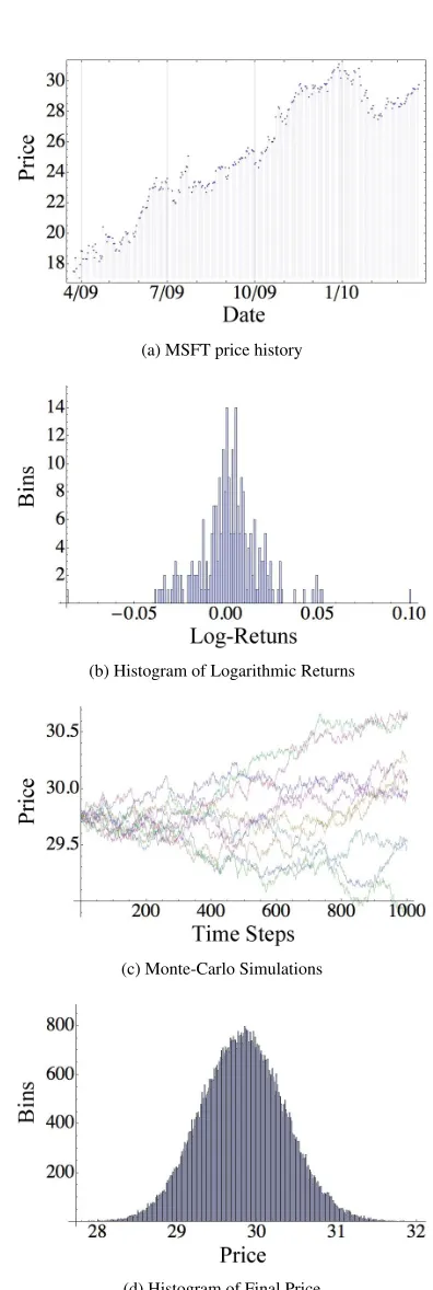
process by using the stock Microsoft (MSFT), which is included in the portfolio of stocks that we are ultimately interested in—the Dow Jones industrial average.
4.1
Historical Drift and Diffusion
Figure 1a shows the closing prices of Microsoft from March 23, 2009 at $17.95 until March 23, 2010 at $29.88. Let this series be{S0, S1, S2, . . . ST}. In this
case,T = 251given the number of trading days in the provided interval. From this data series, we can calculate the relative price changes using
Ri = ln
S
i+1
Si
, 0≤i≤T−1. (1)
Riis called the log (or continuously compounded)
re-turn. It is positive for relative increases in the stock price and negative for decreases. A histogram ofRivalues for
Microsoft is shown in Figure 1b with bin size 0.005. The distribution ofRifor this example is roughly normal, and
any deviation from a normal distribution, as we will now derive, is evidence against the Black-Scholes assumption of asset prices following geometric Brownian motion.
With GBM, asset prices are modelled as
dSt = µStdt+σStdWt. (2)
With a logarithmic transform of St and application of
Ito’s lemma, GBM can be found to have the following analytic solution:8
St = S0exp
µ−σ
2
2
t+σWt
. (3)
Due to theWtterm, this solution is a process. Thus if
we are given a set of(S0, St)pairs, we can estimate the
valuesµandσto fit this process.
Let∆tbe the sampling interval relative to the mea-sured period. For example, if we sample daily prices and want the annualized distribution,∆twould be 251. In our case, we sample daily values to estimate the distri-bution over the same time-period: one day. Thus we use ∆t= 1. From equation 3, the distribution should be
Ri ∼ N
µ−σ
2
2
∆t, σ2∆t
. (4)
By taking our sampled data Ri and computing the
standard deviation, we have an estimate for the daily dif-fusionσ. In finance, this is called the historic volatility (although not all volatility measures are calculated the same way). Next we find the mean ofRi, and estimate
the drift termµas: mean(Ri) +σ2/2. For the MSFT
data, we find the daily drift and diffusion estimators to beµ= 0.23%andσ= 1.77%per day.
8Argument omitted for brevity. See an introductory computational finance textbook,e.g.,[38].
(a) MSFT price history
(b) Histogram of Logarithmic Returns
(c) Monte-Carlo Simulations
(d) Histogram of Final Price
A first note on bias. Recall that the Black-Scholes model assumes that dividends are not paid out. This is not true for historic data. For the example, the MSFT data includes four dividend payments of $0.13 each. This causes the closing price to be adjusted downward. Thus equation 1 should differentiate between pre- and post-adjusted prices: denominatorSishould be the
post-adjusted price for timei, while numeratorSi+1 should
be the pre-adjusted (raw) price for timei+ 1. We found the difference to be insignificant due to dividends being infrequent and small, and thus ignored dividends.
4.2
Monte-Carlo Simulation
With estimates forµandσ, we next consider the distri-bution of outcomes over the time-period,τ, for which we want to harvest entropy. To generate this distribution, we use a Monte-Carlo simulation of the process in equation 3. We discretizeτ, which is one day for the MSFT ex-ample, intomequal-sized steps of size∆τ. Equation 3 can then be simulated as Algorithm 1.
Algorithm 1: A Monte-Carlo trial for simulating as-set price movements.
for(0≤j < m)do
1
t←T+j·∆τ
2
Zt←rN(0,1)
3
St+1←Stexp
µ−σ2
2
∆τ+σZt
4
We begin atST, the last observed price ($29.88 for
MSFT), and map a possible trajectory toST+τ by
step-ping through Algorithm 1. Line 2 simply keeps the timestep notation tidy. Line 3 indicates a random vari-able drawn from a standard normal distribution. This variable is used in the next line, in conjunction with theµ
andσparameters to step the price forward one interval. We then repeat the algorithmN times to generate many independent possible outcomes forST+τ. Figure 1c
il-lustrates the first 10 trajectories, while Figure 1d shows a histogram of outcomes for100 000simulations and a bin size of one cent.
A second note on bias. Generally, Monte-Carlo is sub-ject to three types of error. There is the discretization error due to modelling a continuously random process withmintervals. In our case, the exact solution in line 3 of Algorithm 1 is unbiased by discretization error be-cause it is multiplicative. In models other than GBM, the only known solution may be an additive approximation instead (for example, GBM itself could alternatively be approximated bySt+1=St+Stµ∆τ+StσZtwhich is
called Euler time-stepping). In this latter case, the error
is orderO(m−1). The second source of bias is usingN
trials to estimate some value. In computational finance, the value of interest is the mean of theNoutcomes. With both types of error, we reach the often stated total er-ror of Monte-Carlo methods in computational finance:
O(max(m−1, N−0.5))[38]. However in our case, we
have an exact solution that eliminates the first term, and we are interested in the entropy of the distribution ofN
trials, not the mean, resulting in a different bias for the second term. We will discuss howNinfluences this bias in the next section after we have defined entropy.
The third possible source of bias is the statistical prop-erties of the random number generator used for line 2 of Algorithm 1. We used the default generator in Math-ematica, which we believe is more than sufficient for Monte Carlo simulations. It creates a seed from ses-sional information, uses cellular automata to expand the seed into pseudorandom bits, and Box-Muller to trans-form these into a normally distributed number.9 We also experimented with a Mersenne twister, sometimes rec-ommended for use in computational finance (e.g.,[38]), and it made no significant difference.10
Why use Monte Carlo? Given that we have an exact solution for GBM, in equation 3, we could eliminate the discretization step and generateST+τvalues in a single
step. Instead, we use time-stepping to create an approach that is easily replicable if one were to swap GBM for a different financial model where an exact solution is not known—i.e.,mean reversion or jump-diffusion models. Our aim is to assist the interested reader in studying dif-ferent models.
4.3
Entropy Estimation
We now consider how much entropy is provided in a stock price over the course of a day. We first estimate the Shannon entropy, which provides an average-case mea-sure of unpredictability, as this has the most intuitive ap-peal and highlights parameter dependence well. We later will consider min-entropy, which provides a worst-case measure. The Shannon entropy of discrete random vari-ableX with probability mass function p(x)is defined as
H(X) = −X
x
p(x) log2p(x). (5)
Given the results from the Monte Carlo simulation, we have a list ofN possible outcomes for the price of our
9http://reference.wolfram.com/mathematica/
tutorial/RandomNumberGeneration.html
asset. Denote these outcomes P = {P1, P2, . . . , PN},
wherePiisST+τfor theithMonte Carlo trial. We round
each outcome to the nearest cent and place it in a set of bins for each unique price. Since many trials will yield the same price once rounded, letNˆ ≤Nbe the number of unique outcomes observed (i.e.,non-empty bins). De-finePˆ = hpˆj,Pˆji, for1 ≤ j ≤ Nˆ, as the set of pairs
wherePˆj is a unique price inPandpˆjis the number of
times it appears.
To estimate the Shannon entropy in our set P, we compute
H(P) = −
ˆ
N
X
j=1
ˆ
pj
N log2
ˆ
pj
N
. (6)
This type of estimator is known as a maximum like-lihood, naive, or plug-in estimator [34]. It works by distributing the random variable into bins and estimat-ingp(x)by dividing the number of outcomes in each bin by the total number of outcomes. The goal of this paper is to estimate the entropy of a closing price, rounded to the nearest cent, which is a discrete random variable. So we use a bin size of one cent.
A third note on bias. Maximum likelihood estimators (MLE) for Shannon entropy are biased. As with any ran-dom sampling, some bins may have more values than they theoretically should and others less and this tends to average out asN increases. However for entropy es-timation, an empty bin cannot be included in Equation 6 because0·log(0) is undefined. Instead, empty bins are dropped from the estimate even if theoretically they should be non-empty. This leads to a negative bias for MLE and the entropy is lower than it should be.
In our case, we want a conservative estimate of en-tropy and so negative biases of this sort are not so trou-bling. However the bias can be corrected if we can pro-vide an estimate of how many bins have non-zero prob-ability (relative to the number of samples). To estimate this value, we take the full range ofmin(P)tomax(P). Let this beMˆ bins. The Miller-Madow bias [33] of an MLE is given as
B = ˆ
M−1
2N . (7)
As stated, it is a negative bias and so the adjusted en-tropy is:HB(P) =H(P) +B. Other adjustments exist
in the literature [34]. We selected Miller-Madow because it is computationally easy to compute for large values ofN and appropriate whenN > Mˆ.11 For the MSFT data that we have been using to illustrate each step, we
11More precisely, ifN/Mˆ diverges to∞asNgrows, thenHB(P)
will converge on the correct result.
usedN = 100 000and foundNˆ = 397andMˆ = 447. The MLE Shannon entropy is 7.764 bits and the Miller-Madow bias is 0.002, which is relatively small.
Min-Entropy. While Shannon entropy provides an es-timate of the average entropy in a stock price, a worst-case estimate is needed if we want to extract the ran-domness out of the price. Given a distributionX, the min-entropy,H∞(X), is defined as
H∞(X) = −log2(maxx (p(x))). (8)
In other words, for any possible outcomex,p(x) ≤ 2H∞(X). IfXis uniformly random, the Shannon entropy
and min-entropy are equivalent. Otherwise, min-entropy is strictly less. Since H∞(X)is ultimately computed
from one probability p(x) and this value will be non-zero if the entropy is non-non-zero, the bias from empty bins on Shannon entropy does not apply to the notion of min-entropy.
We use the Shannon entropy estimates to examine the effect of drift, diffusion, initial price, and elapsed-time in the next subsection. We use the min-entropy estimate when we want to configure a random extractor to produce a short, near uniform-random bit-string from the much longer set of prices.
4.4
Experimental Results
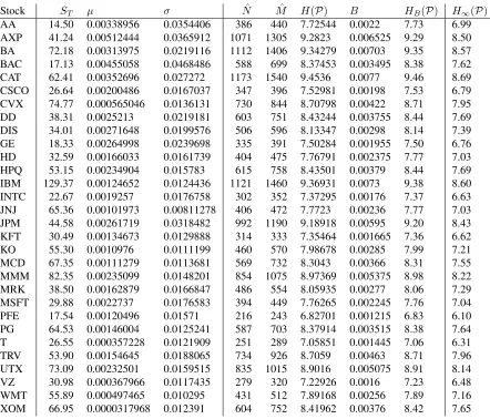
In the Scantegrity II municipal election, a portfolio of 30 stocks was used.12 These stocks were the companies that make up the Dow Jones industrial average (DJIA) — an important financial benchmark. Table 1 shows the data that we collected and our estimates for each of these stocks following the approach outlined for the MSFT ex-ample. The prices were observed from March 23, 2009 to March 23, 2010 (S0toST), and these were used to
es-timate the daily drift and diffusion rates: µandσ. With these parameters, we simulated the path from the clos-ing price on March 23, 2010, ST, forward one day in
time using a Monte Carlo simulation with 100 000 tri-als. The number of unique prices (to the nearest cent) in our simulation,Nˆ, is used to generate an MLE-estimate for the Shannon entropy: H(P). The estimated number of expected non-empty bins,Mˆ, is used to estimate the Miller-Madow bias:B. These are combined to generate our adjusted estimate of Shannon entropy: HB(P).
Fi-nally, we also provide our estimate of the min-entropy:
H∞(P). Pfizer (PFE) had the lowest entropy: 6.83
and 6.10 bits for Shannon and min-entropy respectively, while Caterpillar (CAT) had the highest at 9.46 and 8.69 bits respectively.
12B. Adida. Takoma Park: Meeting 2. http://benlog.com/
Stock ST µ σ Nˆ Mˆ H(P) B HB(P) H∞(P)
AA 14.50 0.00338956 0.0354406 386 440 7.72544 0.0022 7.73 6.99
AXP 41.24 0.00512444 0.0365912 1071 1305 9.2823 0.006525 9.29 8.50
BA 72.18 0.00313975 0.0219116 1112 1406 9.34279 0.00703 9.35 8.57
BAC 17.13 0.00455058 0.0468486 588 699 8.37453 0.003495 8.38 7.62
CAT 62.41 0.00352696 0.027272 1173 1540 9.4536 0.0077 9.46 8.69
CSCO 26.64 0.00200486 0.0167037 347 396 7.52981 0.00198 7.53 6.79
CVX 74.77 0.000565046 0.0136131 730 844 8.70798 0.00422 8.71 7.95
DD 38.31 0.0025213 0.0219181 603 751 8.43244 0.003755 8.44 7.69
DIS 34.01 0.00271648 0.0199576 506 596 8.13347 0.00298 8.14 7.39
GE 18.33 0.00264998 0.0239698 335 391 7.50284 0.001955 7.50 6.76
HD 32.59 0.00166033 0.0161739 404 475 7.76791 0.002375 7.77 7.03
HPQ 53.15 0.00234904 0.015783 615 758 8.43501 0.00379 8.44 7.69
IBM 129.37 0.00124652 0.0124436 1121 1460 9.36931 0.0073 9.38 8.60
INTC 22.67 0.0019257 0.0176758 302 352 7.37295 0.00176 7.37 6.63
JNJ 65.36 0.00101973 0.00811278 406 472 7.7723 0.00236 7.77 7.03
JPM 44.58 0.00261719 0.0318482 992 1190 9.18918 0.00595 9.20 8.43
KFT 30.49 0.00134673 0.0129888 314 333 7.35464 0.001665 7.36 6.62
KO 55.30 0.0010976 0.0111199 460 570 7.98678 0.00285 7.99 7.21
MCD 67.35 0.00111279 0.0113681 569 732 8.3043 0.00366 8.31 7.55
MMM 82.35 0.00235099 0.0148201 854 1075 8.97369 0.005375 8.98 8.22
MRK 38.50 0.00162879 0.0166847 486 554 8.05935 0.00277 8.06 7.29
MSFT 29.88 0.0022737 0.0176583 394 449 7.76265 0.002245 7.76 7.04
PFE 17.54 0.00120496 0.01571 216 243 6.82701 0.001215 6.83 6.10
PG 64.53 0.00146004 0.0125241 587 703 8.37914 0.003515 8.38 7.64
T 26.55 0.000357228 0.0121909 251 289 7.05851 0.001445 7.06 6.31
TRV 53.90 0.00154645 0.0188065 734 926 8.7059 0.00463 8.71 7.96
UTX 73.09 0.00232501 0.0159515 835 1015 8.9016 0.005075 8.91 8.14
VZ 30.98 0.000367966 0.0117435 279 320 7.22926 0.0016 7.23 6.48
WMT 55.89 0.000497465 0.010295 431 512 7.89168 0.00256 7.89 7.16
XOM 66.95 0.0000317968 0.012391 604 752 8.41962 0.00376 8.42 7.65
Table 1: The Dow Jones portfolio of 30 stocks. For the Monte-Carlo parameters, we show: initial price (ST), historic
diffusion parameter (µ), and historic drift parameter (σ). For the Shannon entropy estimate, we show: the number of unique prices in the simulation (Nˆ), the estimated number of non-empty bins (Mˆ), the Shannon entropy estimate based on observed prices (H(P)), the Miller-Madow bias (B), and the bias-adjusted estimate (HB(P)). For the min-entropy
estimate, we show the estimate based on observed prices (H∞(P)).
Drift Diffusion Initial Price Time
µ H(P) σ H(P) ST H(P) τ H(P)
Min 0.003% 6.81 0.81% 8.53 $14.50 7.33 0.5 day 8.03
Mean 0.195% 8.54 1.87% 8.54 $ 48.02 8.54 1 day 8.54
Max 0.513% 9.95 4.68% 8.54 $ 129.37 9.85 2 days 9.03
We were also interested in the individual effect of drift, diffusion, opening price, and time-period on the entropy of a stock. We created a mythical stock with the mean value for each of these parameters, calculated from the DJIA data. The stock hadµ= 0.195%,σ= 1.87%, and
ST = $48.02and was simulated over one day. For each
parameter, we individually varied it to the minimum and maximum observed value for this parameter in the DJIA data and estimated the resulting Shannon entropy. We also varied the timeframe from half a day to two days. The results are provided in Table 2. The entropy was sensitive to the observed spread in bothµ andST but
largely invariant to changes inσ. In all cases, an increase in the parameters resulted in an increase in the entropy.
4.5
Portfolio Entropy
We have shown how to estimate the entropy of individ-ual stocks. But how much entropy is in a collection of stock prices? From Figure 1, it may be tempting to sum the entropy estimates for all the stocks and use this as an estimate of the total entropy in the portfolio. This approach works only if the stocks are uncorrelated with each other. In reality, stocks typically display varying de-grees of correlation with other stocks from, for example, the same business sector, same country, or when traded on the same index. This means that the portfolio entropy is less than the sum of the entropy of the individual stocks due to mutual information between subsets of the stocks. We selected the two stocks with the highest correla-tion and estimated the mutual informacorrela-tion between them. Pairwise throughout the portfolio, the highest correlated stock pairs are Cheveron and Exxon (0.82 over one year) which are both large oil and gas producers. Next are JP Morgan and Bank of America (0.78) which are both large banks. The mean correlation was 0.42.
Taking Cheveron and Exxon (CVX and XOM), we generated correlated Monte Carlo paths [38]. To do this, recall Algorithm 1. We perform this algorithm for CVX. Denote the value ofZt in line 3 for CVX as ZtC. For
XOM, our second stock, we will run almost the same al-gorithm; we replace line 4. First denote the output at line 3 asZX
t and let the correlation between CVX and XOM
beρ. Then the replacement for line 4 is
StX+1←StXexp
µ−σ
2
2
∆τ
+σρZtC+p1−ρ2ZX t
.
(9)
In other words, ZX
t is used as a joint random variable
shared between both stocks.
Using this method, we ran10 000 000trials to estimate the joint Shannon entropy between Exxon and Cheveron.
This was the largest simulation that was computation-ally feasible for us. Recall from Table 1 that the num-ber of unique prices observed for Cheveron and Exxon were respectively 730 and 604. That means the number of unique price pairs is on the order of 730*604. Thus our simulation of 10M trials was only one order of mag-nitude greater than the number of observed events and our result is a quite sparse histogram from which the es-timates will be sufficiently biased. We found that the joint entropy was 15.96 bits compared to the sum of their individual entropies: 16.90 bits. That means the mutual information is at most 0.94 bits. Again, we did not adjust for bias (Miller-Madow is best when the trials are much larger than the outcomes) and so the mutual information is likely less than this. For min-entropy, the result is 1.04 bits.
We leave a rigorous analysis of mutual information in the entire Dow Jones index for future work. As men-tioned, computing the joint entropy between two stocks is very difficult as it is: the number of bins squares, as does the number of trials needed to create a suitably dense histogram. Methods exist for estimating bias when the trials are less than the number of bins [34] but it is not obvious how to extend these estimators to more than two random variables. Computing the joint entropy between 30 stocks does not seem computationally feasible, even if the trials could be less than the resulting bins by a poly-nomial factor.
We can provide a very crude estimate by making a generous assumption. Recall the chain rule for joint en-tropy is as follows:
H(P1,P2, . . . ,Pn) = n
X
i=1
H(Pi|Pi−1, . . . ,P1). (10)
We could estimate theH(Pi|Pi−1, . . .)term for each
stock as: H(Pi)−max(i,j=6 i)(I(Pi,Pj)). This would
hold if the worst-case mutual information between any two stocks in the portfolio was less than the mutual in-formation a given stock has with the rest of the portfo-lio. In other words, any mutual information Cheveron shared with a stock other than Exxon (because of simi-larities in sectors, country, exchange,etc.) would already be accounted for in the mutual information it shares with Exxon. This is crude and the estimate should be treated only as a ballpark figure. For the DJIA under this as-sumption, the Shannon entropy is 218 bits and min-entropy is 192.
5
Beacon Implementation
increases the entropy. In this section, we consider how to convert a list of closing prices into a form that is use-ful for general cryptographic protocols. Since the field of cryptography has conventions in notation that sometimes conflict with conventions in computational finance or in-formation theory, we will, in a small number of cases, redefine variables in this section.
LetPi be a list of closing prices from our portfolio
on dayi. We encode the prices as integers with a fixed, sufficient number of digits and concatenate them: i.e.,
{14.34,41.08, . . .} →001434k004108k. . .. Let the bit-length|Pi|=n. If the prices in the list are, for example,
the 30 stocks of the DJIA, encoding each price with 6 digits will produce a 180 digit or 598 bit string. However from our simulations in the previous section, we estimate that there would be only 218 bits of entropy in this 598 bit string, and 192 extractable bits.13 Because the ran-domness is not concentrated, this semi-random string is not a suitable for seeding selection algorithms or pseu-dorandom generators, or as a cryptographic challenge. In this section, we provide a protocol that, among other things, takes as input a long, semi-random string of stock prices, and output a shorter string of near-uniform ran-dom bits.
The stock market prices can be used in at least one of two ways: it can be sampled directly by any party requir-ing a random challenge, or, alternatively, a neutral third party can regularly sample the source, produce a random bit-string in some useful form, and publish it for quick reference by any party requiring an unpredictable chal-lenge (or seed, common reference string, nonce, etc.). We call such a publisher abeacon service provider(BSP) and we will refer to the random values it produces as
seeds. In general, the BSP will be agnostic of what the seeds are being used for.
A BSP can provide a few benefits: if an election (or other protocol) has a low risk of fraud, the fact the en-tity claims a seed is random may be trustworthy enough. In higher risk protocols, the derivation of the seed can be independently verified and the BSP is not trusted at all. Since the BSP is regularly publishing a new seed, it can update in a recursive fashion, mixing the new clos-ing prices with the previous seed. This makes the output dependent on the prices that preceded it. Finally, as an incentive to provide a beacon service, we can, with care, also allow the BSP to influence the seed with its own ran-domness. This also provides a marginal hedge for every-one else: even if the closing prices are fully manipulated, the attacker will still have to also collude with the BSP to fix the seed.
13Even if we did not prepend each price with as many leading zeros, the entropy would still be less than the length of the string. This is because the most significant digits in the price is much less likely to change than the least significant digit (i.e.,the one cent digit).
5.1
Definitions
Randomness Extractor. Briefly, Extk is a function:
{0,1}n × {0,1}d → {0,1}m. It takes ann-bit input
of sufficient entropy and ad-bit key k and returns an
m-bit output of high entropy wherem < n. Here suffi-cient entropy means the min-entropy of{0,1}nis at least
mbits (we will generally require2m) and high entropy means that the statistical distance between the distribu-tion on{0,1}mandmuniform random bits is, where
is a negligible function inm. We only consider the case whered=m. For a formal definition, see [17].
CBC-MAC. Briefly, CBC-MACis a mode of operation for a block cipher based on cipher block chaining (CBC) with an initialization vector of zero, but it returns only the final block. It is suitable for creating message authenti-cation codes (MAC). Dodiset al. show thatCBC-MACis an extractor if the block cipher is an ideal random per-mutation, the plaintext has2mbits of min-entropy for an
m-bit output, and the key is uniformly random. For the full details (including an upper bound on the input size), see [17].
Pseudorandom Generator. Briefly, G is a function: {0,1}m→ {0,1}l(m). It takes anm-bit seed and returns
a polynomially-bounded number of bitsl(m) typically greater thanm. The distribution on{0,1}l(m)is-close
to uniform random. For a formal definition, see [6].
Robust Pseudorandom Generators. Barak and Halevi provide a construction for a robust pseudo-random generator [6]. A robust PRG uses a standard PRG,G, as well as maintaining some evolving internal state si that can be referenced during operation. G
is cryptographically secure: the internal state cannot be inferred from the output by an adversary bound to probabilistic polynomial time (PPT). The construction separates the task of updating the state from the task of generating pseudorandom bits. We only reference the former function:refresh.
refresh: {0,1}m× {0,1}n→ {0,1}m
si←G(si−1⊕Extk(Pi)).
This function is of interest because it could be used for updating the seeds of a beacon service, where the seed is substituted for the state. A robust PRG affords a number of functions to an adversary. Of interest, badRefreshlets the adversary refresh with a chosenPi,
andsetStateallows the adversary to learnsi and
re-place it with a chosensi+1. In the face of these attacks,
(not needed for a beacon service since past seeds are pub-lic), break-in recovery, and resilience. Briefly, break-in recovery means that if an adversary learnssi for round
i, si+1 is still unpredictable ifrefresh is run with a
sufficiently random Pi+1. Resilience means that if an
adversary controlsPi+1 but does not knowsi, si+1 is
unpredictable.
Bilinear Groups. Let GandGT be cyclic groups of
orderq, whereqis a large prime. Lete:G×G→GTbe
a bilinear, non-degenerate, and efficient mapping. That is, ∀g1, g2 ∈ G and ∀a1, a2 ∈ Zq: e(ga11, g
a2
2 ) =
e(g1, g2)a1·a2 whereeis computable in polynomial time
ande(g, g)generatesGT for someg ∈ G. Finally, as-sume the q-decisional bilinear Diffie-Hellman inversion assumption holds for the group (definition omitted for brevity – see [9]).
Verifiable Unpredictable Function. Briefly, a VUF is a tuple of four functions. GenK returns secret keysk
and public key pk. Evalsk(x) takes input x and
re-turns a unique and unpredictable y (we omit defining the domain and range, as they vary by construction). Proofsk(x, y)returns proofπx,y thatyis the output on
x. Verifypk(x, y, πx,y)returns 1 iff proof is correct.
A VUF is a weaker primitive than a verifiable random function (VRF). Givenx, a VUF guaranteesycannot be guessed with non-negligible advantage, while a VRF of-fers the stronger guarantee thatycannot be distinguished from a random element with non-negligible probability. A VUF is sufficient for us because we know the entropy iny and will use an extractor to convert it into the re-quired form. For a formal definition of both, see [18].
Dodis-Yampolskiy VUF. Dodis and Yampolskiy pro-pose the following VUF, defined over a bilinear group: {G,GT, g ∈ G, q} [18]. GenK publishes the group, randomly generates secret key sk ←r Zq∗ and
pub-lishes public keypk = gsk.
Evalsk(x)takesx ∈ Zq∗
and returns y, which in practice is a point on an ellip-tic curve. Evalsk(x)is defined as y ← g
1 x+sk. The
proof is embedded iny; Proofsk(x, y) simply returns
{x, y}.Verifypk(x, y, πx,y)is defined ase(pk·gx, y)
?
=
e(g, g).
5.2
Security Properties
The central function of our BSP protocol updates the seed at interval iwith new randomness Pi. We define
it with the recurrence: si ← Update(si−1, si−2,Pi),
wheresi is the seed at intervaliandsi−1 andsi−2are
the two preceding seeds. An update function does not need to usetwoprevious seeds—it could be more or less.
The seeds are akin to the internal state of a robust PRG, except that they are made public at each interval. We assume the BSP has a secret key. We have several prop-erties we want from our protocol.
• Verifiable. A polynomial time verifier should be convinced that Update was computed from Pi,
si−1, andsi−2as specified in the protocol.
• Statistically Random. The statistical difference betweensi and a uniform distribution of the same
length should be-close.
• Unpredictable.The advantage of a PPT-bound ad-versary in predicting si without Pi is negligible,
even if the adversary knows si−1, si−2 and the
BSP’s secret key.
• Parisian.The advantage of a PPT-bound adversary in computing the exact value of Pi needed to
out-put a chosensi is negligible ifsi is chosen before
knowingPi−1andsi−1andsi−2, even is she knows
the BSP’s secret key.
• Partially Distributed. The advantage of a PPT-bound adversary in predicting si is negligible if
she knowssi−1andsi−2, choosesPi, but does not
know the BSP’s secret key.
With the exception of the Parisian property, the mo-tivation for these is hopefully intuitive and not in need of further explanation. We will illustrate the last prop-erty with a concrete example. Suppose on the Tuesday night of a given week, election officials post the results of an election and the post-election challenges are to be generated on the Friday of that week after the markets close. On Thursday night, the adversary knows the seed from Thursday and let us assume she can fully manipu-late Friday’s closing prices. Further, assume that she has a particular seed that she wants produced to ensure some fraud committed on Tuesday escapes detection. It should be computationally infeasible for the adversary to deter-mine the closing prices she needs to set in order to gen-erate, from the existing seeds, this target seed she wants. The only way the adversary can produce the desired seed on Friday is to manipulate the prices every day: Wednes-day, ThursWednes-day, and Friday. We name this “parisian” after the Parisian options we discussed earlier, which required a barrier event to occur on multiple days.
5.3
Protocol
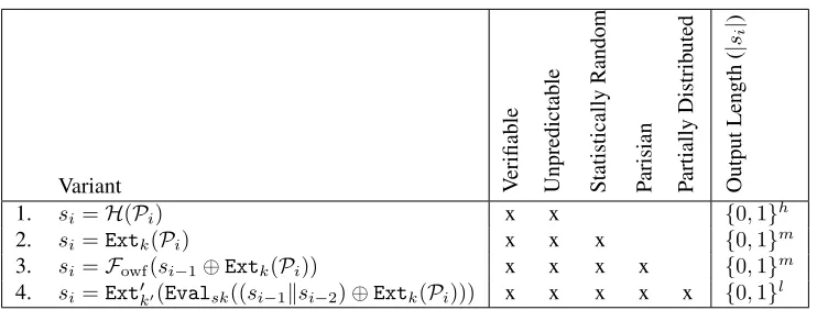
Variants. In this section, we define a protocol that can be used by a BSP to implement theUpdatefunction de-scribed in the previous section. The stock market ran-domness, Pi, is n bits and contains 2m bits of
Variant Verifiable Unpredictable Statistically
Random
P
arisian
P
artially
Distrib
uted
Output
Length
(
|
si
|
)
1. si=H(Pi) x x {0,1}h
2. si=Extk(Pi) x x x {0,1}m
3. si=Fowf(si−1⊕Extk(Pi)) x x x x {0,1}m
4. si=Ext0k0(Evalsk((si−1ksi−2)⊕Extk(Pi))) x x x x x {0,1}l
Table 3: A sequence of intermediate protocols, and which properties they achieve, leading to our suggested protocol. AssumingPihas2mbits of min-entropy, the output length is provided. Lengthhdepends on the hash function used,
whilem= 2l(e.g.,h=160,m=256 andl=128).
output, whileExt0k0has anl-bit key andl-bit output. We
considerm= 2l.
Table 3 shows some related constructions. Perhaps the simplest approach is to publish anh-bit hash of the list of closing prices each day: Variant 1. BeforePiis known,
the hash ofPiwill trivially be unknown as well, and once
Pi is known, anyone can verify the output is correct by
recomputing the hash from their source for the closing prices.
The problem with using a fixed hash function is that it does not guarantee a statistically random output. Dodis
et al.show that even if a hash function is modelled with an ideal compression function (and Merkle-Damgaard chaining), it does not have good extraction properties. Instead, the hash needs to be taken from a family of hash functions (i.e., a keyed hash) and even then, one must pay attention to the padding scheme used to ensure the final block has sufficient entropy [17]. With the use of a proper extractor, Variant 2 of the protocol produces a statistically random output. While extractors are keyed, the key,k, only needs to be uniformly random. Its value is not kept secret and the key can be reused.
Variant 2 is not Parisian because it is only function-ally dependent on the most recent closing prices of the stocks. LetFowf denote a one-way function. Variant 3
adds the Parisian property and is essentially therefresh function of a Barak-Halevi robust PRG. Recallrefresh is defined as: si ← G(si−1⊕Extk(Pi)). Gis used as:
{0,1}m→ {0,1}m(i.e.,there is no expansion ofm) and
PRGs are one-way.14
Variant 4 is our protocol. The main modification is to replaceG(·)with theEvalsk(·)function of a VUF, which
allows the BSP to influence the seed withsk, while
main-14So why isGnot a one-way function in the Barak-Halevi model? The answer is because we are only using one of two functions of-fered by the robust PRG model—the other function uses the sameG
as:{0,1}m→ {0,1}2m.
taining verifiability. This adds the partially distributed property. The other variants were verified by recomput-ing the value. In this case, the BSP produces a correct-ness proof forEvalsk(·)that is checked. The properties
of the VUF also imply that without knowledge ofsk, the output ofEvalsk(·)is unpredictable if the input is
un-known.
VUF Details. A variety of VUFs and VRFs exist. We use the Dodis-Yampolskiy VUF [18] for its simplicity, efficiency, and the fact that its proof is non-interactive.15 However since it is based on bilinear pairings, we re-quire some encoding. Recall the domain ofEvalis an exponent and the range is a point on an elliptic curve. LetΦ1: {0,1}m → Z∗q be an encoding function that is
entropy preserving (i.e.,injective). Whenq > 2m, this
encoding is the trivial one. LetΦ2 be a mapping from
an element inGT → {0,1}m. This encoding (or
ex-traction) is more difficult, and it is specific to the type of elliptic curve used. For a random point on an ordi-nary curve defined overF22l, anl-bit string can be
ex-tracted [23]. For a supersingular curve (which offer fast pairing operations), we are not aware of any specific ex-tractor. Instead, we simply concatenate the coordinates together and use a randomness extractor,Ext0k0, which
produces anl-bit output.
Extractor Details. In deciding on how to implement Extk, we consider two options.
• We could use an approach that is specific to the dis-tribution we are drawing from: closing prices (for the first extraction). For example, we could con-sider a daily relative increase in price as heads and
a decrease as tails. Due to the drift term, there is a slightly biased toward heads which can be corrected for with a Von Neumann extractor—see Footnote 1. However this approach produces less than a bit of entropy per closing price (and therefore does not guarantee even one bit of entropy each day the mar-ket closes) and since stocks are correlated, it is not clear how to use more than one stock.
• Dodis et al. investigate using a block cipher in CBC-MAC mode—the result quoted above. This construction has less “fine-print” than some of the alternatives they examine. If the plaintext has2m
bits of min-entropy and isLblocks long, it produces an m-bit output with a statistical distance, from a uniformly random m-bits, of O(L 2−m/2). A side-benefit is that it also has an “avalanche-effect” where a difference in a single bit of the input causes a random-looking difference in the output. We use this approach.
Key Derivation. The CBC-MAC extractor, or any other non-deterministic extractor, does have one issue however: how it is keyed. Extractor keys do not need to be secret (in fact, for verifiability, they cannot be), how-ever they must be uniformly random. Again, we consid-ered a few options.
• The BSP could choose a uniformly random key at the beginning of the protocol and use it throughout. However this is providing adversarial control over the key, and we cannot cite any strong results on what an adversary could do with this control. • Assuming we can bootstrap the process, we will be
generating good quality randomness at every itera-tion and so we could use the values of the previous seeds to refresh the key to the extractor. The results from the extraction literature assume a uniform ran-dom key and do not indicate if an-close random key is sufficient (or could be compensated for by increasing the entropy of the input).
• We could use the historic prices of a single stock and a Von Neumann extractor as described in the first bullet point of the preceding list. While we re-jected this approach for the extractor itself, it works well for generating a key. Since there are no unpre-dictable or secrecy requirements on the key, we can use past prices instead of future prices. This gives us immediate access to enough bits to generate the two required extraction keys (k andk0). In addi-tion, the key can be continually updated by shifting in new bits as time goes by. We give full details of this key derivation procedure in Appendix A.1 in the full version of the paper.16
16Available at:http://eprint.iacr.org/2010/361
Algorithm 2: Update Beacon
begin
1
xi= (si−1ksi−2)⊕Rijn256-CBC-MACki(Pi)
2
yi=g
1 xi+sk
3
si =AES128-CBC-MACk0 i(yi)
4
end
5
Publish:{yi, si}
6
Algorithm 3: Verify Beacon
begin
1
xi= (si−1ksi−2)⊕Rinj256-CBC-MACki(Pi)
2
e(pk·gxi, y
i)
?
=e(g, g)
3
si
?
=AES128-CBC-MACk0 i(yi)
4
end
5
Protocol. The BSP publishes pairing-friendly {G,GT, g∈G, q}. The BSP choosesskrandomly from
Zq∗ and publishes pk = gsk. The BSP generates the
current extraction keyskiandki0. The initial statess−1
and s0 are set to zero. On day i ≥ 1, BSP takes the
closing stock prices, Pi, and executes Algorithm 2. To
verify thatsi is a proper update tosi−1, a verifier with
{pk, ki, k0i,Pi, yi, si, si−1, si−2} executes Algorithm 3.
Note that the verifier does not need to verify that the seeds from si−1 back in time to s1 were themselves
correctly formed. To be assured that si is a random
beacon, it is sufficient to check it is correctly formed from the arbitrary values claimed to besi−1 andsi−2.
This is becausePifully refreshes the randomness ofsi.
Parameter Sizes. For the extractors, we need a block cipher and AES is the default candidate. However the choice of AES locks us into only using an extractor with 128 bit outputs. If we use Rijndael, we can expand that choice to 128, 192, or 256 bit outputs. Our protocol re-quires two extractors and with each extraction, we lose half of the bits of entropy in the input. Therefore we start with 512 bits of min-entropy inPiand use
Rijndael-25617to generate a valuexiwith (-close to) 256 bits of
min-entropy. These 256 bits are preserved inyiand then
a second extraction with AES-128 produces a value si
with (-close to) 128 bits of min-entropy.
This approach depends onPihaving at least 512 bits
of min-entropy. We estimated the DJIA only has 192 bits. However we have also shown that adding additional stocks increases the total min-entropy. We would like
the portfolio to be easy to construct, and ideally iconic— for this reason, we recommend using the S&P 500. By extrapolating our results, the daily closing prices of these 500 stocks provides 512 bits of min-entropy with a large safety margin.18 This will allow us to produce a fresh 128-bit random number every market day.
This approach also assumes we can encode the 256-bit numberxiinto the subgroup of a pairing-friendly curve.
Common curve sizes, however, work in subgroups of 160-bits and so this would require a custom implementa-tion. If alternative sizes for the extractors are preferable, one could use a variable-length block cipher [4] instead ofRijndael/AES, which allows extractors of any size.19
5.4
Security Analysis (Abstract)
Due to space restrictions, we omit the analysis of secu-rity for our protocol; however, it is included in Appendix A.2-7 of the full version of this paper20. In the analy-sis, we prove that our protocol has the five properties we have specified. We note that some of the properties we want to prove are subsumed by the properties of a Barak-Halevi robust PRG. This includes directly: statistically random and unpredictable (unpredictable is equivalent to their notion of break-in recovery).Parisianis also im-plied but not explicit. However, we prove each of these independently for our variant, plus demonstrating verifi-abilityand thepartially distributedproperty.
6
Concluding Remarks
In this paper, we have shown that the closing prices for common stocks contain sufficient min-entropy for gen-erating random challenges for use in elections or other cryptographic applications. This result, in combination with the ease with which stock prices can be verified, makes financial data an attractive source of randomness for cryptographic voting systems unable to use the Fiat-Shamir heuristic, and possibly for precinct selection in standard electronic voting. In addition to the entropy es-timates, we have provided a provably secure protocol for implementing a beacon service. It is our hope that such a beacon service, whether using our protocol or a variant, becomes a reality.
18This is not meant to suggest that the 30 stocks used by Scantegrity are insufficient. For the number of units to be audited in this election, a seed of 16 bits expanded with a PRNG provides good statistical proper-ties (cf.[12, 36]). As shown, this is nearly achieved by CVX and XOM alone.
19Although thesecurityof these ciphers has not been examined as closely as AES, neither has been examined in any detail for good
extractionproperties.
20Available at:http://eprint.iacr.org/2010/361
Future Work. We list a few items for future work. First, estimating joint entropy between correlated stocks becomes infeasible as the number of stocks grows. Progress on making this estimation more efficient would be welcome. Second, some results concerning extractors built with standard cryptographic primitives would be useful: specific bounds (instead of asymptotic bounds), analysis of using inputs where the min-entropy is less than twice the min-entropy of the output, and analysis of extraction with a key that is only statistically-close to uniform random, instead of being exactly uniform ran-dom. A third item for future work would be alternative VUFs, in particular a scheme that works over the inte-gers, to reduce the complexities of mapping from a finite-field over elliptic curves back to the integers. Ideally, if a VUF mappedm-bit integers tom-bit integers, then the second extractor would not be needed at all.
Acknowledgements. The authors thank the Punchscan and Scantegrity teams for many discussions on the use of financial data as beacons. In particular, we acknowl-edge Ron Rivest for the idea of using the DJIA as an entropy pool and for the protocol used in the Scantegrity II election in Takoma Park. The issue of inconsistent re-porting of stock volumes was raised by Ben Adida and James Heather. We thank Aleks Essex and the anony-mous reviewers for their input on a draft of this paper. The authors acknowledge the support of this research by the Natural Sciences and Engineering Research Council of Canada (NSERC)—the first author through a Canada Graduate Scholarship and the second through a Discov-ery Grant.
References
[1] B. Adida. Helios: web-based open-audit voting. USENIX Secu-rity Symposium 2008.
[2] B. Adida, O. de Marneffe, O. Pereira, and J.J. Quisquater. Elec-tion a university president using open-audit voting.EVT 2009.
[3] R.K. Aggarwal and G. Wu. Stock market manipulation—theory and evidence.Journal of Business, 79(4) 2003.
[4] R.J. Anderson and E. Biham. Two Practical and Provably Secure Block Ciphers: BEARS and LION.FSE 1996.
[5] L. Babai. Trading group theory for randomness.STOC 1985.
[6] B. Barak and S. Halevi. A model and architecture for pseudo-random generation and applications to/dev/random. CCS 2005.
[7] F. Black and M. Scholes. The pricing of options and corporate liabilities.Journal of Political Economy, 81(3), 1973.
[8] M. Blum, P. Feldman, and S. Micali. Non-interactive zero-knowledge and its applications.STOC 1988.
[9] D. Boneh and M. Franklin. Identity-based encryption from the Weil pairing.CRYPTO 2005.
[11] D. Chaum, R. Carback, J. Clark, A. Essex, S. Popoveniuc, R. L. Rivest, P. Y. A. Ryan, E. Shen, and A. T. Sherman. Scantegrity II: end-to-end verifiability for optical scan election systems using invisible ink confirmation codes.EVT 2008.
[12] J. Clark, A. Essex, and C. Adams. Secure and observable auditing of electronic voting systems using stock indices. IEEE CCECE 2007.
[13] J. Calandrino, J.A. Halderman, and E.W. Felten. In defense of pseudorandom sample selection.EVT 2008.
[14] J. Camenisch, S. Hohenberger, M. Kohlweiss, A. Lysyanskaya, and M. Meyerovich. How to win the clone wars: efficient periodic n-times anonymous authentication.CCS 2006.
[15] M. Chesney, M. Jeanblanc-Picque, and M. Yor. Brownian excur-sions and Parisian barrier options.Advances in Applied Probabil-ity, 29, 1997.
[16] A. Cordero, D. Wagner, and D. Dill. The role of dice in election audits.WOTE 2006.
[17] Y. Dodis, R. Gennaro, J. Hastad, H. Krawczyk, and T. Rabin. Randomness extraction and key derivation using the CBC, Cas-cade and HMAC modes.CRYPTO 2004.
[18] Y. Dodis and A. Yampolskiy. A verifiable random function with short proofs and keys.PKC 2005.
[19] D. Eastlake. Publicly Verifiable Nomcom Random Selection. RFC 2777, IETF, 2000. http://www.ietf.org/rfc/ rfc2777.txt
[20] D. Eastlake. Publicly Verifiable Nominations Committee (Nom-Com) Random Selection. RFC 3797, IETF, 2004. http:// www.ietf.org/rfc/rfc3797.txt
[21] A. Essex, J. Clark, R. T. Carback, and S. Popoveniuc. Punchscan in practice: an E2E election case study.WOTE 2007.
[22] S. Even, O. Goldreich, and A. Lempel. A randomized protocol for signing contracts.CACM, 28(6), 1985.
[23] R.R. Farashahi, R. Pellikaan, and A. Sidorenko. Extractors for binary elliptic curves. Designs, Codes, and Cryptography, 49, 2008.
[24] A. Fiat, and A. Shamir. How to prove yourself: practical solutions to identification and signature problems.CRYPTO 1986.
[25] S. Goldwasser and Y. Kalai. On the (in)security of the Fiat-Shamir paradigm.FOCS 2003.
[26] S. Goldwasser and M. Sipser. Private coins versus public coins in interactive proof systems.STOC 1986.
[27] J. Groth and A. Sahai. Efficient non-interactive proof systems for bilinear groups.EUROCRYPT 2008.
[28] A. Halderman and B. Waters. Harvesting verifiable challenges from oblivious online sources.CCS 2007.
[29] J.L. Hall. On improving the uniformity of randomness with Alameda County’s random selection process. 2008.
[30] D. Jefferson, E. Ginnold, K. Midstokke, K. Alexander, P. Stark, and A. Lehmkuhl (State of California’s Post-Election Audit Stan-dards Working Group). Evaluation of Audit Sampling Models and Options for Strengthening Californias Manual Count. Report, 2007.
[31] A. Juels, M Jakobsson, E. Shriver, and B. Hillyer. How to Turn Loaded Dice into Fair Coins.IEEE Transactions on Information Theory, 46(3), 2000.
[32] R. Merton. Theory of rational option pricing.Journal of Eco-nomics and Management Sciences, 4(1), 1973.
[33] G. Miller. Note on the bias of information estimates. “Information Theory in Psychology II-B.” Free Press, 1955.
[34] L. Paninski. Estimation of entropy and mutual information. Neu-ral Computation, 15, 2003.
[35] M. Rabin. Transaction protection by beacons.Journal of Com-puter and System Sciences, 27(2), 1983.
[36] E. Rescorla. On the security of election audits with low entropy randomness.EVT 2009.
[37] M. Schroder. Brownian excursions and Parisian barrier options: a note.Advances in Applied Probability, 40(4), 2003.
[38] R.U. Seydel. “Tools for computational finance.” Springer, 4th ed, 2009.
[39] B. Waters, A. Juels, J. A. Halderman, and E. W. Felten. New client puzzle outsourcing techniques for DOS resistance. CCS 2004.