Simulation based security in the applied pi calculus
St´ephanie Delaune1, Steve Kremer1, and Olivier Pereira2 1
LSV, ENS Cachan & CNRS & INRIA, France 2
UCL Crypto group, Belgium
Abstract. We present a symbolic framework for refinement and composition of security protocols. The framework uses the notion of ideal functionalities. These are abstract systems which are secure by construction and which can be combined into larger systems. They can be separately refined in order to obtain concrete pro-tocols implementing them. Our work builds on ideas from computational models such as the universally composable security and reactive simulatability frame-works. The underlying language we use is the applied pi calculus which is a general language for specifying security protocols. In our framework we can ex-press the different standard flavours of simulation-based security which happen to all coincide. We illustrate our framework on an authentication functionality which can be realized using the Needham-Schroeder-Lowe protocol. For this we need to define an ideal functionality for asymmetric encryption and its realization. We also show a joint state result for this functionality which allows composition (even though the same key material is reused) using a tagging mechanism.
1
Introduction
Symbolic techniques showed to be a very useful approach for the modeling and analysis of security protocols: for twenty years, they improved our understanding of security pro-tocols, allowed discovering flaws [18], and provided support for protocol design [11]. These techniques also resulted in the creation of powerful automated analysis tools [5, 10, 3], and impacted on several protocol standards used every day, e.g., [9].
Until now, symbolic techniques mostly concentrated on specifying and proving con-fidentiality and correspondence properties, i.e., showing which symbols are kept secret, and on which session parameters participants agree when a protocol session completes. However, such specifications do not provide any information about the behavior of pro-tocols when they are used in composition with other propro-tocols, and surprising behaviors are well know to happen in such contexts [8]. Moreover, protocols are often expected to provide more sophisticated security guarantees: we can think of privacy-type properties for voting protocols, or input independence for auction protocols.
can be successively refined into more concrete protocols, but also composed to build more complex protocols. Functionalities have been proposed for a wide range of proto-col tasks, including general secure multi-party computation [6]. In the spi-calculus [2], Abadi and Gordon also present the idea of a protocol being equivalent to an idealized version. This is however more restrictive as they do not have the notion of a simulator.
Simulation-based security frameworks can typically be decomposed into two “lay-ers”: (i) a foundational layer that provides a general model for concurrent computation, and (ii) a security layer that provides general security definitions, most importantly the notion of secure protocol emulation to be used. While the security layer is essentially common to all frameworks [4, 6, 7, 15, 19], including this paper, the foundational layer varies widely. Those variations typically lie in the concurrency model (from the most common token-passing mechanism to the use of scheduler with various powers) and in the definition of computational bounds. These differences typically result in incompa-rable security notions.
Defining simulation-based security while choosing the applied pi calculus [1] as the foundational layer brings the main benefits of this approach into the symbolic world:
– it provides a powerful machinery that can be used to specify a wide range of so-phisticated protocol tasks in terms of the behavior of functionalities, and
– general composition theorems guarantee that protocols keep behaving as expected when executed in arbitrary contexts.
While we tried to stick to the common definitions from the security layer of simulation-based security frameworks, the use of the applied pi calculus as foundational layer raised interesting challenges.
First, at the most foundational level, one has to adopt a notion of indistinguishabil-ity of processes. While the symmetric notions of computational indistinguishabilindistinguishabil-ity and observational equivalence are most commonly used in the cryptographic and symbolic worlds respectively, the symmetry of such relations appeared to be too restrictive for our purpose. For instance, requiring a symmetric equivalence relation makes visible the addition of an adversary that simply acts as a relay. Such undesired behaviors moti-vate the introduction of new notions of observational preorder and labelled simulation relations in the applied pi calculus.
Next, our attempts at translating ideal functionalities from the computational world into the symbolic world showed to be a non immediate task. For instance, traditional ideal functionalities for asymmetric encryption produce ciphertexts by encrypting ran-dom strings unrelated to the original messages. In our setting we use a technique of double-encrypting messages such that a plaintext corresponding to a given ciphertext can only be retrieved through the decryption services offered by the functionalities.
2
The applied pi calculus
The applied pi calculus [1] is a language for describing concurrent processes and their interactions.
2.1 Syntax and informal semantics
To describe processes, one starts with a set of names (which are used to name com-munication channels or other atomic data), a set of variables, and a signatureΣwhich consists of the function symbols which will be used to define terms. In the case of se-curity protocols, typical function symbols will includeencfor encryption, which takes plaintext and a key and returns the corresponding ciphertext, anddecfor decryption, taking ciphertext and a key and returning the plaintext. Terms are defined as names, variables, and function symbols applied to other terms. Terms and function symbols are sorted, and of course function symbol application must respect sorts and arities. By the means of an equational theoryEwe describe the equations which hold on terms built from the signature. We denote=Ethe equivalence relation induced byE. Two terms are related by=Eonly if that fact can be derived from the equations inE. When the set of variables occurring in a termT is empty, we say thatT is ground.
Example 1. LetEencbe the theory made up of the equationsdec(enc(x, k), k) =xand
test(enc(x, y), y) =ok. We have thattest(dec(enc(enc(n, k1), k2), k2), k1) =Eok. In the applied pi calculus, one has plain processes and extended processes. Plain processes are built up in a similar way to processes in the pi calculus, except that mes-sages can contain terms (rather than just names). Below,M andN are terms,nis a name,xa variable anduis a metavariable, standing either for a name or a variable. Extended processes add active substitutions and restriction on variables.
P, Q, R:= plain processes 0
P |Q νn.P
ifM =NthenP elseQ in(u, x).P
out(u, N).P
A, B, C:=extended processes
P A|B νn.A νx.A {M/
x}
{M/
x}is the substitution that replaces the variablexwith the termM. Active sub-stitutions generalise “let”. The process νx.({M/
x} | P) corresponds exactly to the process “letx=M inP”. As usual, names and variables have scopes, which are de-limited by restrictions and by inputs. We writefv(A),bv(A),fn(A)andbn(A)for the sets of free and bound variables and free and bound names ofA, respectively. We also assume that, in an extended process, there is at most one substitution for each variable, and there is exactly one when the variable is restricted. We say that an extended process is closed if all its variables are either bound or defined by an active substitution.
Active substitutions are useful because they allow us to map an extended processA
a frameϕ, denoted bydom(ϕ), is the set of variables for whichϕdefines a substitution (those variables xfor whichϕcontains a substitution{M/
x}not under a restriction on x). An evaluation context C[ ] is an extended process with a hole instead of an extended process.
Example 2. Consider the following processP:
νk.(in(io1, x).out(net,enc(x, k))
|in(net, y).iftest(y, k) =okthenout(io2,dec(y, k))else0).
The first component receives a messagexon the channelio1and sends its encryp-tion with the keykon the channelnet. The second is waiting for an inputyonnet, uses the secret keykto decrypt it. If the decryption succeeds, then it forwards the resulting plaintext onio2.
2.2 Semantics
The operational semantics of processes in the applied pi calculus is defined by structural rules defining two relations: structural equivalence (briefly described in Section 2.1) and internal reduction, noted→. Structural equivalence, noted≡, is the smallest equiv-alence relation on extended processes that is closed underα-conversion on names and variables, application of evaluation contexts, and some other standard rules such as associativity and commutativity of the parallel operator and commutativity of the bind-ings. In addition the following three rules are related to active substitutions and equa-tional theories:
νx.{M/
x} ≡0, {M/x} |A≡ {M/x} |A{M/x}, and{M/x} ≡ {N/x} ifM =EN
Internal reduction→is the smallest relation on extended processes closed under structural equivalence and application of evaluation contexts such that
COMM out(a, M).P |in(a, x).Q→P |Q{M/ x}
THEN ifM =NthenPelseQ→P whereM =EN
ELSE ifM =NthenPelseQ→Q
for any ground termsM andN such thatM 6=EN
The operational semantics is extended by a labelled operational semantics enabling us to reason about processes that interact with their environment. Labelled operational semantics defines the relation−→α whereαis either an inputin(a, M)(ais a channel name andM is a term that can contain names and variables), orνx.out(a, x) (xis variable of base type), orout(a, c)orνc.out(a, c)(cis a channel name). We adopt the following rules in addition to the internal reduction rules:
IN in(a, x).P−−−−−→in(a,M) P{M/x}
OUT-CH out(a, c).P−−−−−→out(a,c) P
OPEN-CH A
out(a,c)
−−−−−→A′ c6=a
νc.A−−−−−−−→νc.out(a,c) A′
OUT-T out(a, M).P−−−−−−−→νx.out(a,x) P| {M/ x}
x6∈fv(P)∪fv(M)
SCOPE A
α
−→A′ udoes not occur inα νu.A−→α νu.A′
bn(α)∩fn(B) =∅
PAR A
α
−→A′ bv(α)∩fv(B) =∅ A|B−→α A′|B
STRUCT A≡B B
α
Our rules differ slightly from those described in [1], although we prove in [12] that labelled bisimulation in our system coincides with labelled bisimulation in [1].
Example 3. Consider the processPdefined in Example 2. We have that:
P −−−−−→in(io1,s) νk.(out(net,enc(s, k))
|in(net, y).iftest(y, k) =okthenout(io2,dec(y, k))else0)
−→ νk.iftest(enc(s, k), k) =okthenout(io2,dec(enc(s, k), k))else0)
−→ νk.out(io2, s) νx.out(io
2,x)
−−−−−−−−→ νk.{s/ x}
LetAbe the resulting process. We have thatφ(A)≡νk.{s/ x}.
2.3 Equivalences
In [1], it is shown that observational equivalence coincides with labelled bisimilarity. This relation is like the usual definition of bisimilarity, except that at each step one additionally requires that the processes are statically equivalent.
Definition 1 (static equivalence (≈s)). Two termsM andN are equal in the frame
φ, written(M =E N)φ, if, and only if there exists n˜ and a substitutionσsuch that
φ ≡νn.σ˜ ,M σ =EN σ, andn˜∩(fn(M)∪fn(N)) =∅. Two framesφ1 andφ2are statically equivalent,φ1 ≈s φ2, whendom(φ1) = dom(φ2), and for all termsM, N we have that(M =EN)φ1if and only if(M =EN)φ2.
Example 4. Letϕ0=νs.{enc(s,k)/x}andϕ1 =νr.{r/x}wherek, sandrare names and E be the theory given in Example 1. We have (test(x, k) =E ok)ϕ0 but not
(test(x, k) =Eok)ϕ1, thusϕ06≈sϕ1. However, we haveνk.ϕ0≈sϕ1.
We are now defining observational equivalence and observational preorder. For this we introduce the notion of a barb. Given an extended processAand a channel namea, we writeA⇓awhenA →∗ C[out(a, M).P]for some termM, plain processP, and
evaluation contextC[ ]that does not binda.
Definition 2 (observational preorder, equivalence). Observational preorder () (resp. equivalence (≈)) is the largest (resp. largest symmetric) relation on extended processes having same domain such thatARBimplies
1. ifA⇓athenB ⇓a;
2. ifA→∗A′, thenB →∗B′andA′RB′for someB′;
3. C[A]RC[B]for all closing evaluation contextsC[ ].
Definition 3 (labelled (bi)similarity). A relationRon closed extended processes is a simulation relation ifARBimplies
1. φ(A)≈sφ(B),
2. ifA→A′, thenB →∗ B′andA′RB′for someB′,
3. ifA →α A′ andfv(α)⊆dom(A)andbn(α)∩fn(B) =∅, thenB →∗→→α ∗ B′
IfRandR−1are both simulation relations we say thatRis a bisimulation relation. Labelled similarity (ℓ), resp. labelled bisimilarity (≈ℓ), is the largest simulation, resp. bisimulation relation.
Observational preorder and similarity were not introduced in [1]. However, these definitions seem natural for our purposes. Obviously we have that≈ ⊂ and≈ℓ⊂ ℓ. We now show that labelled bisimilarity is a precongruence.
Proposition 1. LetAandBbe two extended processes such thatA ℓ B. We have thatC[A]ℓC[B]for all closing evaluation contextC[ ].
From this proposition it follows thatℓ⊆ . Hence, we can use labelled similarity as a convenient proof technique for observational preorder. We actually expect the two relations to coincide but did not prove it as we did not need it. Moreover, the relationℓ is stable under application of replication and replication distributes over parallel.
Lemma 1. LetP andQbe two closed plain processes. We have that: (i) ifP ℓ Q then!P ℓ!Q; (ii)!(P |Q) ℓ!P |!Qand!P |!Q ℓ!(P |Q).
3
Simulation based security
3.1 Basic definitions
The simulation-based security approach classically distinguishes between input-output channels, which yield the internal interface of a protocol or functionality to its environ-ment and network channels, which allow the adversary to interact with the functionality. We suppose that all channels are of one of these two sorts:IOorNET. Moreover the sort system ensures that names of sortNETcan never be conveyed as data on a channel, i.e. these channels can never be transmitted. We writefnet(P)forfn(P)∩NET.
Definition 4 (functionality, adversary). A functionalityF is a closed plain process. An adversary forFis an evaluation contextA[ ]of the form:
νgnet1.(A1|νgnet2.(A2|. . .|νgnetk.(Ak| ). . .))withfnet(F)⊆S1≤i≤kgneti⊆NET where eachAi(1≤i≤k) is a closed plain process, andfn(A[ ])∩IO=∅.
We may note that ifA[ ]is an adversary forFthenfnet(A[ ]) =fnet(A[F]).
Lemma 2. LetF be a functionality andA1[ ]be an adversary for F. Then A1[F] is a functionality. Besides, if A2[ ] is an adversary forA1[F], thenA2[A1[ ]]is an adversary forF.
While adversaries can control the communications of functionalities onNET chan-nels, IO contexts model the environment of those functionalities, providing them with their inputs and collecting their outputs.
Definition 5 (IO context). An IO context is an evaluation contextCio[ ]of the form νioe1.(C1 | νioe2.(C2 | . . .|νioek.(Ck | ). . .))with S1≤i≤kioei ⊆IOwhere eachCi (1≤i≤k) is a closed plain process.
3.2 Strong simulatability
The notion of strong simulatability [16], which is probably the simplest secure emula-tion noemula-tion used in simulaemula-tion-based security, can be formulated in our setting.
Definition 6 (strong simulatability). LetF1andF2be two functionalities.F1 emu-lates F2 in the sense of strong simulatability, written F1 ≤SS F2, if there exists an adversarySforF2(the simulator) such thatfnet(F1) =fnet(S[F2])andF1S[F2]. The definition ensures that any behavior ofF1can be matched byF2executed in the presence of a specific adversaryS. Hence, there are no more attacks onF1 than attacks onF2. Moreover, the presence ofS allows abstract definitions of higher-level functionalities, which are independent of a specific realization.
Example 5. LetFcc=in(io1, s).out(netcc,ok).in(netcc, x).ifx=okthenout(io2, s). The functionality models a confidential channel and takes a potentially secret valuesas input on channelio1. The adversary is notified via channelnetccthat this value is to be transmitted. If the adversary agrees the value is output on channelio2. This functional-ity can be realized by the processP introduced in Example 2.
LetS=νnetcc.in(netcc, x).νr.out(net, r).in(net, x).ifx=rthenout(netcc,ok)| ). We indeed have thatPℓS[Fcc]andfnet(P) =fnet(S[Fcc]).
In order to examine the properties of strong simulatability in our specific setting, we now define a particular adversary which is called a dummy adversary.
Definition 7 (dummy adversary). Let F be a functionality. The dummy adversary forFis the adversaryD[ ] =νsim.g(D1|νgnet.(D2| ))where:
– gnet=fnet(F) ={net1, . . . ,netn}; – simg={simi
1, . . . ,simin,simo1, . . . ,simon} ⊆NET;
– D1= !in(net1, x).out(simi1, x)|. . .|!in(netn, x).out(simin, x)|
!in(simo1, x).out(net1, x)|. . .|!in(simon, x).out(netn, x); – D2= !in(sim1i, x).out(net1, x)|. . .|!in(simin, x).out(netn, x)|
!in(net1, x).out(simo1, x)|. . .|!in(netn, x).out(simon, x); By construction we have thatfnet(D[F]) =fnet(F).
Lemma 3. LetFbe a functionality andD[ ]the dummy adversary forF:F D[F].
However, we do not have thatF ≈ D[F], sinceD[F]has more non-determinism thanF. A direct consequence of this lemma is thatF1 F2andfnet(F1) =fnet(F2) implies that F1 ≤SS F2: it is sufficient to observe that F2 D[F2]and hence by transitivityF1D[F2]. We use these observations to show that≤SSis a preorder. Lemma 4. The relation≤SS is a preorder, that is the following hold: (i) reflexivity:
F1≤SS F1; (ii) transitivity:F1≤SS F2andF2≤SSF3 ⇒ F1≤SSF3.
Proposition 2. LetF1,F2be functionalities andCiobe an IO context. F1≤SS F2 =⇒ Cio[F1]≤SS Cio[F2].
Now, we prove the following composition results. Actually, closure under parallel composition of functionalities is a direct consequence of the previous proposition by noticing that whenF is a functionality then | F is an IO-context. The proof of the closure under replication is more involved and given in Appendix.
Proposition 3. LetF1,F2andF3be three functionalities. We have that: (i)F1≤SS F2 ⇒ F1| F3≤SSF2| F3; and (ii)F1≤SSF2 ⇒!F1 ≤SS!F2.
3.3 Other notions of simulation based security
Several other notions of simulation based security appear in the literature. We present these notions, and show that they all coincide in our setting. This coincidence is typi-cally regarded as highly desirable [16, 15], while it does not hold in most simulation-based security frameworks [6, 4].
Definition 8. LetF1andF2be two functionalities andAbe any adversary forF1. – F1 emulatesF2 in the sense of black box simulatability, writtenF1 ≤BB F2, iff
∃S.∀A.A[F1] A[S[F2]]whereSis an adversary forF2withfnet(S[F2]) =fnet(F1). – F1 emulates F2 in the sense of universally composable simulatability, written
F1 ≤UC F2, iff ∀A.∃S.A[F1] S[F2] whereS is an adversary forF2 such thatfnet(A[F1]) =fnet(S[F2]).
– F1emulatesF2in the sense of universally composable simulatability with dummy adversary, writtenF1 ≤UCDA F2, iff∃S. D[F1] S[F2]whereDis the dummy adversary forF1andSis an adversary forF2such thatfnet(S[F2]) =fnet(D[F1]).
Theorem 1. We have that≤SS =≤BB=≤UC=≤UCDA.
The above security notions can also be defined replacing observational preorder by observational equivalence. We denote the corresponding relations by ≤SS
≈,≤BB≈ ,≤UC≈
and≤UCDA
≈ . Surprisingly, the use of observational equivalence turns out to be too strong,
ruling out natural secure emulation cases: for instance, the≤SS
≈ relation is not reflexive.
4
Applications
We use the notationin(u,=M)to test whether the input onuis equal (moduloE) to the termM (if not, the process blocks). We sometimes use tuples of terms, denoted byhM1, . . . , Mni, while keeping the equational theory for these tuples implicit. Lastly, we omit “elseQ” in a conditional whenQ= 0.
4.1 Asymmetric encryption with joint state
In this section we introduce a functionality for asymmetric encryption together with a joint state composition result which is crucial for composition of protocols that share key material. Even though encryption in a Dolev-Yao model is already idealized we will see that we nevertheless need to introduce an ideal functionality for encryption in order to obtain the joint state composition result. Throughout this section we rely on the following equational theory:
adec(aenc(x,pk(y), z), y) =x testdec(aenc(x,pk(y), z), y) =ok.
The first equation models randomized asymmetric encryption whereas the second one allows testing whether decryption with a given key succeeds or not.
Real encryption. The real encryption functionality is described in Figure 1:
– Initialisation: the functionality receives a channel nameio1pke, which will be used for all sensitive information exchanges, i.e. when this functionality is used the chan-nelio1pke should be restricted. A fresh private keyskis generated and the corre-sponding public key, i.e.pk(sk), is sent onio1pke. Then the process is ready to re-ceive encryption or decryption requests. Note that encryption requests can be sent on the sensitive channelio1pkeor on the public channelio2pkewhich is the channel the environment will typically use. Decryption requests are only available through the sensitive channelio1pkeand thus will not be used by the attacker.
– EncryptionPenc: each time this process receives a request on the channel io1pke (resp.io2pke), it computes the corresponding ciphertext (probabilistic encryption) and outputs the ciphertext on the channelio1pke(resp.io2pke).
– DecryptionPdec: each time this process receives a request on the channelio1pke, it tries to decrypt the ciphertext and checks whether the tag isTAG0. If so, it outputs the plaintext on the channelio1pke. Otherwise, it does nothing.
Ppke:=in(iopke,io1pke).νsk.out(io 1
pke,hKEY,pk(sk)i).
(letioi
pke=io 1
pkein!Penc | letio
i
pke=io 2
pkein!Penc |!Pdec)
Penc:=in(io
i
pke,h=ENC, mi).
νr2.letmenc=aenc(hTAG0, mi,pk(sk), r2)inout(io
i
pke,hCIPHER, menci)
Pdec:=in(io1pke,h=DEC, mi).
leth=TAG0, m1i=adec(m, sk)inout(io 1
pke,hPLAIN, mi)
Ideal functionality. We now propose, in Figure 2, an idealized versionFpkeof the real encryption functionality, which guarantees that the confidentiality of messages is pre-served independently of any cryptanalytic effort that could be performed on ciphertexts from the knowledge of public keys. In various cryptographic settings [4, 6, 17], this is achieved by computing ciphertexts as the encryption of random messages instead of the actual plaintext. To be able to perform decryption, a table for plaintext/ciphertext asso-ciations is maintained. The burden of this association table is avoided in our symbolic specification by using two layers of encryption: messages are first encrypted using a secure keypk(ssk), then tagged and encrypted with the public keypk(sk)that is pub-lished during the initialization step. We stress that neitherpk(ssk)norssk are ever transmitted byFpke, guaranteeing that it is impossible to decrypt such a ciphertext out-side the functionality, even if the keyskis adversarially chosen, which will be a crucial feature for our joint state composition theorem.
The ideal functionality behaves as follows:
– Initialisation: the attacker chooses the secret keyskand the tag that will be added in each encryption. Then a secure keysskis generated and now the process is ready to receive encryption or decryption requests.
– EncryptionFenc: each time the process receives a request on the channelio1pke (resp.io2pke), it computes the corresponding ciphertext and outputs the ciphertext on the channelio1pke(resp.io2pke). As explained above, the plaintextmis first encrypted usingpk(ssk)before being tagged and encrypted withpk(sk).
– DecryptionFdec: each time the process receives a request on the channelio1pke, it tries to decrypt the ciphertext and checks if the tag is the tag provided during the initialization. Then, it checks if the resulting plaintext is encrypted underpk(ssk). If so, this means that this ciphertext has been produced by the encryption func-tionality and thus has to be decrypted twice. Otherwise, the ciphertext has been produced by the attacker and the plaintext is sent on the channelio1pke.
Fpke:=in(iopke,io1pke).out(net,INIT).in(net,h=ALGO, sk, tagi).out(io 1
pke,hKEY,pk(sk)i). νssk.(letioi
pke=io 1
pkein!Fenc | letio
i
pke=io 2
pkein!Fenc |!Fdec)
Fenc :=in(io
i
pke,h=ENC, mi).νr1.νr2.
letalea=aenc(m,pk(ssk), r1)in letmenc=aenc(htag, aleai,pk(sk), r2)in out(ioi
pke,hCIPHER, menci) Fdec :=in(io
1
pke,h=DEC, mi).leth=tag, m1i=adec(m, sk)in iftestdec(m1, ssk) =okthenout(io
1
pke,hPLAIN,adec(m1, ssk)i) elseout(io1
pke,hPLAIN, m1i)
Fig. 2: Ideal encryption functionality
Realization. We indeed have that the real encryption functionality realizes the ideal one, i.e.,Ppke ≤SS Fpke. This is witnessed by the adversary:
Composition with joint state. While ≤SS is stable under replication this is not al-ways sufficient to obtain composition guarantees. Indeed replication of a process also replicates all key generation operations. In order to obtain self-composition and inter-protocol composition with common key material we need a joint state functionalityPjs, i.e. a functionality that realizes!Fpkewhile reusing the same key material. We actually show such a functionality for the functionalityFpke, which is a variant ofFpkein which each message is tagged. More precisely, the processFpkeis defined asFpke, except that:
(i) the functionality begins with the instructionsin(iopke,io1pke).in(io1pke, sid)instead of
in(iopke,io1pke), (ii) each input of the formin(c, m)is replaced byin(c,h=sid, mi), and (iii) each output of the formout(c, m)is replaced byout(c,hsid, mi).
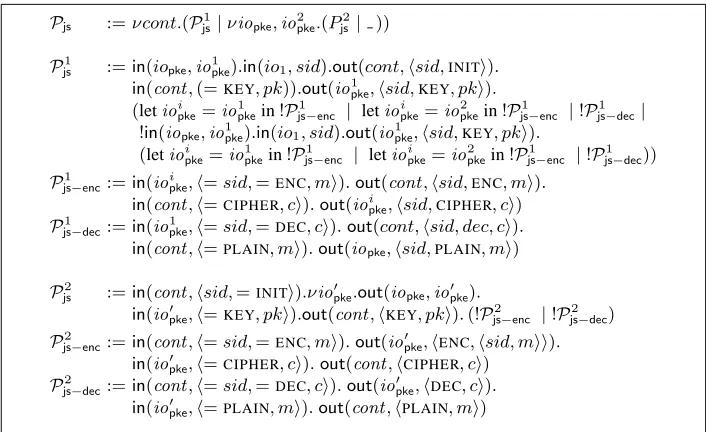
ThePjs functionality process launches one instance of theFpkefunctionality that will be used in all protocol sessions. All the requests to the joint state functionality are received on the public channeliopkein processPjs1. They are then forwarded using the private IO channelcont toP2
js. The processPjs2 shares the private channel iopke withFpkeand forwards all the requests after concatenating the session identifier to the plaintext. Then the response is again forwarded to the processP1
js which outputs the result on the public channeliopke.
Pjs :=νcont.(P 1
js|νiopke,io 2 pke.(P
2 js | ))
P1
js :=in(iopke,io 1
pke).in(io1, sid).out(cont,hsid,INITi). in(cont,(=KEY, pk)).out(io1
pke,hsid,KEY, pki).
(letioipke=io 1 pkein!P
1
js−enc | letio
i
pke=io 2 pkein!P
1
js−enc |!P 1 js−dec|
!in(iopke,io1pke).in(io1, sid).out(io 1
pke,hsid,KEY, pki).
(letioipke=io 1 pkein!P
1
js−enc | letio
i
pke=io 2 pkein!P
1
js−enc |!P 1 js−dec))
P1
js−enc:=in(io
i
pke,h=sid,=ENC, mi).out(cont,hsid,ENC, mi). in(cont,h=CIPHER, ci).out(ioipke,hsid,CIPHER, ci) P1
js−dec:=in(io 1
pke,h=sid,=DEC, ci).out(cont,hsid, dec, ci). in(cont,h=PLAIN, mi).out(iopke,hsid,PLAIN, mi)
P2
js :=in(cont,hsid,=INITi).νio′pke.out(iopke,io′pke). in(io′
pke,h=KEY, pki).out(cont,hKEY, pki).(!P 2
js−enc |!P 2 js−dec)
P2
js−enc:=in(cont,h=sid,=ENC, mi).out(io′pke,hENC,hsid, mii). in(io′
pke,h=CIPHER, ci).out(cont,hCIPHER, ci)
P2
js−dec:=in(cont,h=sid,=DEC, ci).out(io′pke,hDEC, ci). in(io′
pke,h=PLAIN, mi).out(cont,hPLAIN, mi)
Fig. 3: Joint state IO-context
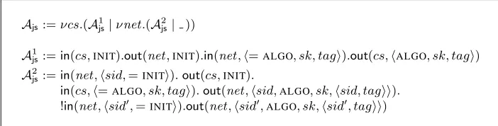
We now observe that the following joint state composition result holds. One instance of the encryption functionality can be used to emulate an unbounded number of such instances using the joint state process:Pjs[Fpke] ≤SS!Fpke.
same keysk. However, note that the session identifiersidused to tag each encryption associated could be different. The value of these session identifiers is selected by the attacker.
Ajs:=νcs.(A 1
js|νnet.(A 2 js| ))
A1
js:=in(cs,INIT).out(net,INIT).in(net,h=ALGO, sk, tagi).out(cs,hALGO, sk, tagi)
A2
js:=in(net,hsid,=INITi).out(cs,INIT).
in(cs,h=ALGO, sk, tagi).out(net,hsid,ALGO, sk,hsid, tagii).
!in(net,hsid′,=
INITi).out(net,hsid′,
ALGO, sk,hsid′, tagii)
Fig. 4: Joint state adversary
Note that it is crucial to introduce the ideal functionality. We indeed have that
Pjs[Ppke] ≤SS Pjs[Fpke] ≤SS !Fpke as well as!Ppke ≤SS!Fpke (wherePpke is de-fined fromPpkein the same way asFpke fromFpke). However,Pjs[Ppke] 6≤SS !Ppke. In particular!Ppke will provide multiple public keys whilePjs[Ppke] only provides a single one. Taking the more abstract ideal functionality allows this to be avoided by a simulator that chooses the same secret key for each instance of the functionality.
4.2 Mutual authentication
Ideal functionality for mutual authentication. TheFauthfunctionality is described in Figure 5 and works as follows. Both the initiator (Finit) and the responder (Fresp) receive a request for mutual authentication on theiriochannel. They forward this request to the adversary and, if both parties are honest, to a trusted hostFthwhich compares these requests and authorizes going further if they match. Eventually, when the adversary asks to finish the protocol, then both participants complete the protocol session.
Realization of mutual authentication. The realization ofFauthbased on the Needham-Schroeder-Lowe protocol is described in Figure 6. For simplicity we consider only two honest identities (ID-AandID-B) and one adversary identity (ID-I). We suppose that these are the only terms of sortidand that the type system only allows these values for the variablesidi. The public key infrastructure is modelled as local tables of the partic-ipants which are used to retrieve the channel names associated to theFpkefunctionality of a given identity. We defineFX
pke to beFpkeX[iopke 7→ iopkeX ]where[iopke 7→ ioXpke] denotes the replacement ofiopkebyioXpke.
We have thatPnsl≤SS Fauthby showing thatPnsl S[Fauth]whereS=νnet.( |
νio2
Fauth:=νc1.νc2.(Finit| Fresp| Fth)
Finit :=in(io1,hINIT, sid, id1, id2i).out(net,hINIT, sid, id1, id2i). ifid2=ID-Ithenin(net,hFINISH,=sid,=id1,=id2i).
out(io1,hfinish, sid, id1, id2i) elseout(c1,hCOMPARE, sid, id1, id2i).
in(c1,h=OK,=sid,=id1,=id2i). in(net,hFINISH,=sid,=id1,=id2i). out(io1,hFINISH, sid, id1, id2i)
Fresp :=in(io2,hINIT, sid, id1, id2i).out(net,hINIT, sid, id1, id2i). ifid1=ID-Ithenin(net,hFINISH,=sid,=id1,=id2i).
out(io2,hFINISH, sid, id1, id2i) elseout(c2,hCOMPARE, sid, id1, id2i).
in(c2,h=OK,=sid,=id1,=id2i). in(net,hFINISH,=sid,=id1,=id2i). out(io2,hFINISH, sid, id1, id2i)
Fth :=in(c1,h=COMPARE, sid, id1, id2i).in(c2,h=COMPARE,=sid,=id1,=id2i). out(c1,hOK, sid, id1, id2i).out(c2,hOK, sid, id1, id2i)
Fig. 5: Mutual authentication functionality
4.3 From one to many sessions
We have shown thatPnsl≤SS Fauth. This result only shows thatPnslis as secure asFauth for a single session of the protocol. By Proposition 3 we have that!Pnsl≤SS!Fauthbut this does not correspond to the expected security for an unbounded number of sessions, as each session uses a different key. To show that!Fauthcan be realized with shared key material we use our joint state result. To apply this result we need the following technical lemma.
Lemma 5. Letnbe a name andcbe a channel name such thatc6∈fn(P)∪fn(Q).
νc.![νn.(out(c, n)|P)|in(c, x).Q] ℓ!νc.[νn.(out(c, n)|P)|in(c, x).Q].
Applying this lemma twice on!Pnslwe obtain that
νioApke,ioBpke.! (FA
pke| FpkeB |νio a
pke,iobpke.
(out(iopke,ioapke)|out(iopke,iobpke)| Pinit| Presp))
≤SS!P nsl
Applying Lemma 1 we have that
νioApke,ioBpke.(!FA
pke|!FpkeB |!νioapke,iobpke.
(out(iopke,ioapke)|out(iopke,iobpke)| Pinit| Presp))
≤SS!P nsl
Now we can use the joint state result to obtain that:
νioA
pke,ioBpke.(PjsA[FpkeA]| PjsB[FpkeB ]|!νioapke,iobpke.
(out(iopke,ioapke)|out(iopke,iobpke)| Pinit| Presp))
≤SS!P nsl
wherePX
Pnsl :=νio
A
pke,ioBpke,ioapke,iobpke.
(Fpke
A | Fpke
B
|out(iopke,ioa
pke)|out(iopke,io
b
pke)| Pinit| Presp)
Pinit :=in(io1,hINIT, sid, id1, id2i). ifid1=ID-Athen letioinitpke=io
a
pkeinP 1 init else ifid1=ID-Bthen letioinitpke=io
b
pkeinP 1 init
P1
init :=ifid2=ID-Athen letio resp pke =io
a
pkeinP 2 init
else ifid2=ID-Bthen letioresppke =io
b
pkeinP 2 init
else ifid2=ID-Ithen letioresppke =ioi
pkeinP 2 init
P2
init :=out(io init pke, sid).
(*Msg 1*) νna.out(ioresppke,hsid,ENC,hna, id1ii).in(ioresppke,h=sid,=CIPHER, x1i). out(netnsl, x1).
(*Msg 2*) in(netnsl, x2).
out(ioinitpke,hsid,DEC, x2i).in(ioinitpke,h=sid,=PLAIN,h=na, ynb,=id2ii). (*Msg 3*) out(ioresppke,hsid,ENC, ynbi).in(ioresppke,h=sid,=CIPHER, x3i).
out(netnsl, x3).
out(io1,hFINISH, sid, id1, id2i)
Presp:=in(io2,h=INIT, sid, id1, id2i). ifid1=ID-Athen letioinit
pke=io
a
pkeinP 1 resp else ifid1=ID-Bthen letioinitpke=io
b
pkeinP 1 resp else ifid1=ID-Ithen letio
i
pke=io
i
pkeinP 1 resp
P1
resp:=ifid2=ID-Athen letio resp pke =io
a
pkeinP 2 resp else ifid2=ID-Bthen letioresppke =io
b
pkeinP 2 resp
P2
resp:=out(io resp pke, sid).
(*Msg 1*) in(netnsl, x1).out(ioresppke,hsid,DEC, x1i).in(ioresppke,h=sid,=PLAIN,hxna,=id1ii). (*Msg 2*) νnb.out(ioinitpke,hsid,ENC,hxna, nb, id1ii).in(ioinitpke,h=sid,=CIPHER, x2i).
out(netnsl, x2). (*Msg 3*) in(netnsl, x3).out(io
resp
pke,hsid,DEC, x3i).in(io resp
pke,h=sid,=PLAIN, ynbi). ifynb=nbthenout(io2,hFINISH, sid, id1, id2i)
Fig. 6: Mutual authentication realization
5
Conclusions
This paper proposes a symbolic framework for the analysis of security protocols along the lines of the simulation based security approach, while adopting the applied pi cal-culus as basic layer. We state central definitions and security notions, show general composition theorems and specific joint-state composition results for asymmetric en-cryption, and illustrate their use in the analysis of a mutual authentication protocol.
calculus and has been integrated in automatic provers, the automation of proofs relying on labeled simulation appears as an interesting challenge for future works.
References
1. M. Abadi and C. Fournet. Mobile values, new names, and secure communication. In Proc.
28th ACM Symp. on Principles of Programming Languages (POPL’01). ACM, 2001.
2. M. Abadi and A. D. Gordon. A calculus for cryptographic protocols: The spi calculus. Technical Report 149, SRC, 1998.
3. A. Armando et al. The AVISPA Tool for the automated validation of internet security protocols and applications. In Proc. 17th Int. Conference on Computer Aided Verification
(CAV’05), LNCS. Springer, 2005.
4. M. Backes, B. Pfitzmann, and M. Waidner. The reactive simulatability (RSIM) framework for asynchronous systems. Information and Computation, 205(12):1685–1720, 2007. 5. B. Blanchet. An Efficient Cryptographic Protocol Verifier Based on Prolog Rules. In Proc.
14th IEEE Computer Security Foundations Workshop (CSFW’01), 2001.
6. R. Canetti. Universally composable security: A new paradigm for cryptographic protocols. In Proc. 42nd IEEE Symp. on Foundations of Computer Science (FOCS’01), 2001. 7. R. Canetti, L. Cheung, D. Kaynar, N. Lynch, and O. Pereira. Compositional security for
Task-PIOAs. In Proc. 20th Computer Security Foundations Symposium (CSF’07), 2007. 8. R. Canetti and J. Herzog. Universally composable symbolic analysis of mutual
authentica-tion and key exchange protocols. In Proc. Theory of Cryptography Conference (TCC’06), LNCS. Springer, 2006.
9. I. Cervesato, A. Jaggard, A. Scedrov, J.-K. Tsay, and C. Walstad. Breaking and fixing public-key kerberos. Information and Computation, 206(2-4):402–424, 2008.
10. C. Cremers. The Scyther Tool: Verification, falsification, and analysis of security protocols. In Proc. 20th Int. Conference on Computer Aided Verification (CAV’08), LNCS, 2008. 11. A. Datta, A. Derek, J. C. Mitchell, and D. Pavlovic. Abstraction and refinement in protocol
derivation. In Proc. 17th IEEE Computer Security Foundations Workshop (CSFW’04), 2004. 12. S. Delaune, S. Kremer, and M. D. Ryan. Symbolic bisimulation for the applied pi-calculus. In Proc. 27th Conference on Foundations of Software Technology and Theoretical Computer
Science (FSTTCS’07), LNCS. Springer, 2007.
13. O. Goldreich, S. Micali, and A. Wigderson. How to play any mental game: A completeness theorem for protocols with honest majority. In Proc. 19th ACM Symposium on the Theory of
Computing (STOC’87). ACM Press, 1987.
14. J. D. Guttman and F. J. Thayer. Protocol independence through disjoint encryption. In Proc.
13th IEEE Computer Security Foundations Workshop (CSFW’00), 2000.
15. R. K¨usters. Simulation-Based Security with Inexhaustible Interactive Turing Machines. In
Proc. 19th IEEE Computer Security Foundations Workshop (CSFW’06), 2006.
16. R. K¨usters, A. Datta, J. C. Mitchell, and A. Ramanathan. On the relationships between notions of simulation-based security. Journal of Cryptology, 21(4):492–546, 2008. 17. R. K¨usters and M. Tuengerthal. Joint State Theorems for Public-Key Encryption and Digitial
Signature Functionalities with Local Computation. In Proc. 21st IEEE Computer Security
Foundations Symposium (CSF’08), 2008.
18. G. Lowe. An attack on the Needham-Schroeder public key authentication protocol.
Infor-mation Processing Letters, 56(3):131–133, 1995.
19. P. Mateus, J. Mitchell, and A. Scedrov. Composition of cryptographic protocols in a proba-bilistic polynomial-time calculus. In Proc. 14th Conference on Concurrency Theory
A
Proof of Proposition 1
The proof relies on the following two lemmas.
Lemma 6. LetRbe the relation on closed extended processes defined as follows:
R= ℓ ∪ {(A, B)|A≡A˜| {M/x}, B≡B˜ | {M/x}, andA˜ℓB˜}.
We have thatRis a labelled simulation.
Proof. LetAandBbe two closed extended processes such thatARB. EitherAℓ
B and we easily conclude. Otherwise, we have that there exist two closed extended processesA˜,B˜, an active substitution{M/x}such that:
A≡A˜| {M/x},B≡B˜ | {M/x}, andA˜ℓB˜.
We show that the 3 points of the definition of labelled simulation hold.
1. A ≈s B. Indeed, we have thatA˜ ≈s B˜, thusA˜ | {M/x} ≈s B˜ | {M/x}. The result easily follows.
2. IfA→A′thenB →∗B′for someB′such thatA′ RB′.
SinceA≡A˜| {M/x}, we have thatA′ ≡A˜′ | {M/x}for some closed extended
processA˜′ such thatA˜ →A˜′. SinceA˜
ℓ B˜, we know that there exists a closed extended processB˜′ such thatB˜ →∗ B˜′ andA˜′
ℓ B˜′. LetB′ = ˜B′ | {M/x}. We have thatB≡B˜ | {M/x} →∗B˜′ | {M/x}def=B′andA′ RB′by definition
ofR.
3. IfA−→α A′withfv(α)⊆dom(A)andbn(α)∩fn(B) =∅, thenB →∗−→→α ∗ B′
for someB′such thatA′ RB′.
SinceA≡A˜| {M/x}, we have thatA′ ≡A˜′ | {M/x}for some closed extended
processA˜′such thatA˜−→α′ A˜′withα′ =α[x7→M]. Note thatfv(α′)⊆dom( ˜A)
and we can assume thatbn(α′)∩fn( ˜B) =∅. SinceA˜
ℓ B˜, we know that there
exists a closed extended processB˜′such thatB˜ →∗−→→α′ ∗B˜′andA˜′
ℓB˜′. Let
B′= ˜B′| {M/x}. We have thatB ≡B˜ | {M/x} →∗−→→α ∗ B˜′| {M/x}def= B′
andA′RB′by definition ofR. This allows us to conclude. ⊓⊔
Lemma 7. LetRbe the relation on closed extended processes defined as follows:
R= ℓ ∪ {(A, B)|A≡νu.˜( ˜A|P), νu.˜( ˜B|P), andA˜ℓB˜}.
We have thatRis a labelled simulation.
Proof. LetAandBbe two closed extended processes such thatARB. EitherAℓB and we easily conclude. Otherwise, we have that there exist two closed extended pro-cessesA˜,B˜, a plain processP (withfv(P)⊆dom(A)) and a sequence of metavari-ablesu˜such that:
We show that the 3 points of the definition of labelled simulation hold. First, we have thatA ≈s B. Indeed, we have thatA˜ ≈s B˜, thus since≈sis closed by application of evaluation context, we deduce thatνu.˜( ˜A|P)≈sνu.˜( ˜B |P), and thusA ≈s B. Now, we distinguish several cases depending on the form of the labelαinvolved in the reductionA−→α A′.
1. α=νx.out(c, x). We distinguish two cases:
(a) A′ ≡νu.˜( ˜A′ |P)for some closed extended processA˜′andA˜−−−−−−−→νx.out(c,x) A˜′
withc, x6∈u˜. (Note thatc, x6∈u˜can be assumed w.l.o.g.: fromA≡νu.˜( ˜A| P), B ≡ νu.˜( ˜B | P)andA˜ ℓ B˜ we obtain by α-conversion thatA ≡
νu˜1.( ˜A1 |P1),B ≡νu˜1.( ˜B1 | P1)for someu˜1withc, x6∈u˜1and asℓis closed under injective renaming of free names we have thatA˜1ℓB˜1). SinceA˜ ℓ B˜, we know that there exists a closed extended processB˜′ such
thatB˜ →∗−−−−−−−→→νx.out(c,x) ∗ B˜′andA˜′
ℓB˜′. LetB′ =νu.˜( ˜B′ |P). We have
thatB ≡νu.˜( ˜B |P)→∗−−−−−−−→→νx.out(c,x) ∗νu.˜( ˜B′ |P)def= B′andA′RB′by
definition ofR.
(b) A′ ≡νu.ν˜ n.˜( ˜A|P′ | {M/x})for some plain processP′and some sequence
of namesn˜such thatn∩˜ fn( ˜B) =∅andP −−−−−−−→νx.out(c,x) ν˜n.(P′ | {M/x})with c, x6∈u˜∪n˜.
LetB′=νu.ν˜ n.˜( ˜B|P′ | {M/x}). We have thatA˜| {M/x}
ℓB˜| {M/x} thanks to Lemma 6 and the fact thatA˜ℓB˜. ThusA˜′ RB˜′by definition of
R. We have also that:
B≡νu.˜( ˜B|P)→∗−−−−−−−→→νx.out(c,x) ∗νu.ν˜ n.˜( ˜B|P′ | {M/x})def=B′.
2. α=out(c, a). We distinguish two cases:
(a) A′ ≡νu.˜( ˜A′ |P)andA˜−−−−−→out(c,a) A˜′witha, c6∈˜u.
SinceA˜ ℓ B˜, we know that there exists a closed extended processB˜′ such
thatB˜ →∗−−−−−→→out(c,a) ∗ B˜′ andA˜′
ℓ B˜′. LetB′ = νu.˜( ˜B′ | P). We have
thatB ≡ νu.˜( ˜B | P) →∗−−−−−→→out(c,a) ∗ νu.˜( ˜B′ | P)def= B′ andA′ RB′ by
definition ofR.
(b) A′ ≡νu.˜( ˜A|P′)andP−−−−−→out(c,a) P′witha, c6∈u˜.
LetB′ =νu.˜( ˜B | P′). By definition ofR, we have thatA˜′ RB˜′. We have
also thatB≡νu.˜( ˜B|P)→∗−−−−−→→out(c,a) ∗νu.˜( ˜B |P′)def= B′.
3. α=in(c, M). We distinguish two cases:
(a) A′ ≡νu.˜( ˜A′ |P)andA˜−−−−−→in(c,M) A˜′withc6∈u˜andu˜do not occur inM.
SinceA˜ℓB˜andfv(M)⊆dom(A)⊆dom( ˜A), we know that there exists a
closed extended processB˜′such thatB˜→∗−−−−−→→in(c,M) ∗B˜′andA˜′
ℓB˜′. Let
B′ =νu.˜( ˜B′ |P). We have thatB ≡νu.˜( ˜B |P)→∗−−−−−→→in(c,M) ∗ νu.˜( ˜B′ | P)def= B′andA′RB′by definition ofR.
(b) A′ ≡νu.˜( ˜A|P′)andP−−−−−→in(c,M) P′withc6∈u˜andu˜do not occur inM.
LetB′ =νu.˜( ˜B | P′). By definition ofR, we have thatA˜′ RB˜′. We have
4. α=νa.out(c, a)anda6∈fn(B). We distinguish four cases:
(a) A′ ≡νu.˜( ˜A′ | P)andA˜−−−−−−−→νa.out(c,a) A˜′withc 6∈u˜. We have also to assume
thata6∈fn( ˜B). (Note again that we can assume this w.l.o.g.: ifa6∈fn(B)and
a6∈ u˜then we can assume thata6∈ fn( ˜B). We can always assumea 6∈u˜as explained previously.)
SinceA˜ℓB˜anda6∈fn( ˜B), we know that there exists a closed extended
pro-cessB˜′such thatB˜ →∗−−−−−−−→→νa.out(c,a) ∗B˜′ andA˜′
ℓ B˜′. LetB′ =νu.˜( ˜B′ |
P). We have thatB ≡νu.˜( ˜B |P)→∗−−−−−−−→→νa.out(c,a) ∗νu.˜( ˜B′|P)def= B′and A′ RB′by definition ofR.
(b) A′ ≡νu.˜( ˜A|P′)andP−−−−−−−→νa.out(c,a) P′withc6∈u˜.
LetB′ =νu.˜( ˜B | P′). By definition ofR, we have thatA˜′ RB˜′. We have
also thatB≡νu.˜( ˜B|P)→∗−−−−−−−→→νa.out(c,a) ∗νu.˜( ˜B|P′)def=B′.
(c) A′ ≡νu˜′.( ˜A′ |P)andA˜−−−−−→out(c,a) A˜′withc6∈u˜,a∈u˜andu˜′ = ˜ur{a}.
SinceA˜ ℓ B˜, we know that there exists a closed extended processB˜′ such
thatB˜ →∗−−−−−→→out(c,a) ∗ B˜′ andA˜′
ℓ B˜′. LetB′ = νu˜′.( ˜B′ | P). We have
thatB ≡νu.˜( ˜B|P)→∗−−−−−−−→→νa.out(c,a) ∗νu˜′.( ˜B′ |P)def=B′ andA′ RB′by
definition ofR.
(d) A′ ≡νu˜′.( ˜A|P′)andP−−−−−→out(c,a) P′withc6∈u˜,a∈u˜andu˜′= ˜ur{a}.
LetB′ =νu˜′.( ˜B | P′). By definition ofR, we have thatA′ RB′. We have
also thatB≡νu.˜( ˜B|P)→∗−−−−−−−→→νa.out(c,a) ∗νu˜′.( ˜B|P′)def= B′.
5. α=τ. We distinguish 8 cases: (a) A′ ≡νu.˜( ˜A′ |P)andA˜→A˜′.
SinceA˜ ℓ B˜, we know that there exists a closed extended processB˜′ such thatB˜ →∗ B˜′ andA˜′
ℓ B˜′. Let B′ = νu.˜( ˜B′ | P). We have that B ≡
νu.˜( ˜B|P)→νu.˜( ˜B′|P)def=B′andA′RB′by definition ofR.
(b) A′ ≡νu.˜( ˜A|P′)andP→P′.
LetB′ =νu.˜( ˜B | P′). By definition ofR, we have thatA′ RB′. We have
also thatB≡νu.˜( ˜B|P)→νu.˜( ˜B|P′)def=B′.
(c) A′ ≡νu.˜( ˜A′ |P′)withA˜−−−−−→out(c,a) A˜′andP −−−−→in(c,a) P′.
SinceA˜ ℓ B˜, we know that there exists a closed extended processB˜′ such
thatB˜ →∗−−−−−→→out(c,a) ∗ B˜′ andA˜′
ℓ B˜′. LetB′ = νu.˜( ˜B′ | P′). We have
thatB ≡ νu.˜( ˜B | P) →∗ νu.˜( ˜B′ | P′) def= B′ andA′ RB′ by definition
ofR.
(d) A′ ≡νu, a.˜ ( ˜A′|P′)withA˜−−−−−−−→νa.out(c,a) A˜′andP−−−−→in(c,a) P′.
SinceA˜ℓB˜anda6∈fn( ˜B), we know that there exists a closed extended
pro-cessB˜′such thatB˜ →∗−−−−−−−→→νa.out(c,a) ∗B˜′andA˜′
ℓB˜′. LetB′=νu, a.˜ ( ˜B′ |
P′). We have thatB ≡νu.˜( ˜B |P)→∗νu, a.˜ ( ˜B′ |P′)def= B′ andA′ RB′
by definition ofR.
SinceA˜ ℓ B˜, we know that there exists a closed extended processB˜′ such
thatB˜→∗−−−−→→in(c,a) ∗B˜′andA˜′
ℓB˜′. LetB′=νu.˜( ˜B′|P′). We have that
B≡νu.˜( ˜B|P)→∗νu.˜( ˜B′|P′)def=B′andA′RB′by definition ofR.
(f) A′ ≡νu, a.˜ ( ˜A′|P′)withA˜−−−−→in(c,a) A˜′andP −−−−−−−→νa.out(c,a) P′.
SinceA˜ ℓ B˜, we know that there exists a closed extended processB˜′ such
thatB˜ →∗−−−−→→in(c,a) ∗ B˜′andA˜′
ℓ B˜′. LetB′ =νu, a.˜ ( ˜B′ | P′). We have
thatB ≡ νu.˜( ˜B | P) →∗ νu.˜( ˜B′ | P′) def= B′ andA′ RB′ by definition
ofR.
(g) A′ ≡νu, x.˜ ( ˜A′ |P′)withA˜−−−−−−−→νx.out(c,x) A˜′andP −−−−→in(c,x) P′.
SinceA˜ ℓ B˜, we know that there exists a closed extended processB˜′ such
thatB˜ →∗−−−−−−−→→νx.out(c,x) ∗ B˜′andA˜′
ℓ B˜′. LetB′ =νu, x.˜ ( ˜B′ | P′). We
have thatB ≡ νu.˜( ˜B | P) →∗ νu, x.˜ ( ˜B′ | P′) def= B′ andA′ R B′ by
definition ofR.
(h) A′ ≡ νu.ν˜ ˜n.( ˜A′ | P′) withA˜ −−−−−→in(c,M) A˜′ andP −−−−−−−→νx.out(c,x) ν˜n.(P′ | {M/x}).
SinceA˜ ℓ B˜ andfv(M) ⊆ fv(P) ⊆ dom(A) ⊆ dom( ˜A), we know that
there exists a closed extended processB˜′such thatB˜ →∗−−−−−→→in(c,M) ∗ B˜′and ˜
A′
ℓB˜′. LetB′ = νu.ν˜ n.˜ ( ˜B′ | P′). We have thatB ≡ νu.˜( ˜B | P) →∗
νu.ν˜ n.˜( ˜B′ |P′)def= B′andA′ RB′by definition ofR. ⊓⊔
Proposition 1. LetAandB be two extended processes such thatA ℓ B. We have thatC[A]ℓC[B]for all closing evaluation contextC[ ].
Proof. We prove this result by structural induction onC[ ]. Base case:C= . In such a case we easily conclude.
Induction step. We distinguish several cases depending on the form ofC.
– C[ ] =νu.C′[ ]. In such a case, thanks to our induction hypothesis, we have that C′[A]
ℓC′[B]. Then, thanks to Lemma 7, we easily deduce thatC[A]ℓC[B]. – C[ ] =P |C′[ ]. We conclude as in the previous case.
– C[ ] ={M/x} |C′[ ]. In such a case, thanks to our induction hypothesis, we have
thatC′[A]
ℓ C′[B]. Then, thanks to Lemma 6, we easily deduce thatC[A] ℓ
C[B].
This allows us to conclude the proof. ⊓⊔
B
Proofs of Section 3
Proof. We define the following relationRon closed extended processes
R = ℓ ∪ {(A, D[A]) | ∃F.fnet(A)⊆fnet(F)and,
D[ ]is a dummy adversary forF}.
We now show thatRis a labelled simulation. IfA ℓ B we trivially conclude. Suppose thatB=D[A]andD[ ]is a dummy adversary for some functionalityFsuch thatfnet(A) ⊆fnet(F). We have thatD[ ] =νsim.g(D1 |νgnet.(D2 | ))whereD1 andD2are closed plain processes as described in Definition 7.
We note that by the type system, for any labelαwe have thatbn(α)∩NET=∅. Hence, ifA(→∗−→→α ∗)∗A′thenfnet(A′)⊆fnet(A). We now show the 3 points of the
definition of a labelled simulation.
1. By construction ofD[ ], we have thatφ(A)≡φ(D[A]), thusφ(A)≈sφ(D[A]). 2. Suppose thatA → A′. As→is closed under application of evaluation contexts,
we have thatD[A] → D[A′]. Moreover,fnet(A′) ⊆ fnet(A). We conclude that A′RD[A′].
3. Suppose thatA→α A′withfv(α)⊆dom(A)andbn(α)∩fn(D[A]) =∅. We have
to consider different cases.
– Names in gnet do not occur in α. In this case D[A] →α D[A′]. Moreover, fnet(A′)⊆fnet(A). We conclude thatA′RD[A′].
– α=in(netk, M). We have that
D[A] ≡ νsim.g(in(netk, x).out(simik, x)|D1|νgnet.(D2|A)) in(netk,M)
−−−−−−−→ νsim.g(out(simik, M)|D1|νgnet.(D2|A))
≡ νsim.g(out(simki, M)|D1|νgnet.(in(simik, x).out(netk, x)|D2|A))
→ νsim.g(D1|νgnet.(out(netk, M)|D2|A))
→ νsim.g(D1|νgnet.(D2|A′))
≡ D[A′]
Moreover,fnet(A′)⊆fnet(A). We conclude thatA′ RD[A′].
– α= (νu.)out(netk, u). We have that
D[A] ≡ νsim.g(D1|νgnet.(in(netk, x).out(simko, x)|D2|A))
→ νsim.g(D1|νgnet.(νu.)(out(simok, u)|D2|A′))
≡ νsim.g(in(simok, x).out(netk, x)|D1|νgnet.(νu.)(out(simok, u)|D2|A′))
→ νsim.g(νu.)(out(netk, u)|D1|νgnet.(D2|A′)) (νu.)out(netk,u)
−−−−−−−−−−→νsimg.(D1|νgnet.(D2|A′))
≡ D[A′]
Moreover,fnet(A′)⊆fnet(A). We conclude thatA′ RD[A′].
Lemma 4. The relation≤SS is a preorder, that is the following hold: (i) reflexivity:
Proof. Reflexivity holds thanks to Lemma 3. Now, it remains to establish transitivity. AsF1≤SSF2andF2≤SSF3, we have that there exist an adversaryS1forF2and an adversaryS2forF
3such that:
– F1 S1[F2]andfnet(F1) =fnet(S1[F2]); – F2 S2[F3]andfnet(F2) =fnet(S2[F3]).
Asis closed under application of evaluation contexts (Proposition 1) we also have thatS1[F
2] S1[S2[F3]]. By transitivity ofwe have thatF1 S1[S2[F3]]. Asfnet(F2) = fnet(S2[F3])andS1is an adversary forF2, we deduce thatS1is also an adversary forS2[F
3]and thus, thanks to Lemma 2, we deduce thatS1[S2[ ]] is an adversary for F3. In order to conclude, it remains to show that fnet(F1) =
fnet(S1[S2[F 3]]).
Asfnet(F2) = fnet(S2[F3]), we deduce thatfnet(S1[F2]) = fnet(S1[S2[F3]]) and we conclude thanks to the fact thatfnet(F1) =fnet(S1[F2]). ⊓⊔
Lemma 8. Letcbe a channel of typeNETandAbe an extended process:νc.AA.
Proof. Actually, we prove a stronger statement. We show that:
AℓB implies νc.AℓB for anyc∈NET.
LetR = ℓ∪ {(A, B) | A ≡ νc.A,¯ A¯ ℓ B}. We show thatRis a labelled simulation. IfAℓBthen we trivially conclude. SupposeARBandA≡νc.A¯with
¯
AℓB. We need to show the 3 points of the definition of labelled simulation.
1. Asc ∈NET, we have thatφ(νc.A¯) ≡φ( ¯A). AsA¯ ℓ B we have thatA¯ ≈s B and hence we conclude thatA≈sB.
2. SupposeA→A′. Henceνc.A¯→A′. By inspection of the reduction rules we have
thatA′≡νc.A¯′andA¯→A¯′for some closed extended processA¯′. AsA¯
ℓBwe have that there existsB′such thatB→∗B′andA¯′
ℓB′. HenceA′RB′. 3. SupposeA −→α A′. Hence,νc.A¯ −→α A′. By the type system we have thatα 6=
νd.out(a, d)for anyd ∈ NET. By inspection of the labelled rules we have that
A′ ≡νc.A¯′ andA¯ −→α A¯′ for some closed extended processA¯′. AsA¯
ℓ Bwe have that there existsB′such thatB→∗−→→α ∗B′andA¯′
ℓB′. HenceA′RB′.
To prove Lemma 8 we observe thatA ℓ A. From the above statement we have that
νc.AℓAand henceνc.AA. ⊓⊔
Note that Lemma 8 relies on the type system and the fact that channels of typeNET
only appear in “channel position”. In particular this avoids a counterexample where
A = out(a, c). In such a case, we have thatA −−−−−→out(a,c) 0, whereas νc.Acan only moves with a label of the formνd.out(a, d).
Proof. AsF1 ≤SS F2we have that there exists a simulatorSforF2such thatF1
S[F2]and fnet(F1) = fnet(S[F2]). As is closed under application of evaluation contexts we also have thatCio[F1] Cio[S[F2]]. By Definition 5 and Definition ??, we have thatCio andSare of the form:
– Cio = νioe1.(C1 | νioe2.(C2 | . . .|νioeℓ.(Cℓ | ). . .))with [
1≤i≤ℓ e
ioi ⊆ IOand
where eachCi(1≤i≤ℓ) is a closed plain process.
– S=νgnet1.(S1|νgnet2.(S2|. . .|νgnetk.(Sk| ). . .)),fnet(F2)⊆ [
1≤j≤k g
netj⊆NET,
fn(S[ ])∩IO=∅and where eachSj(1≤j≤k) is a closed plain process.
Let D[ ] = νsim.g(D1 | νgnet.(D2 | ))be the dummy adversary for Cio[S[F2]]. Thanks to Lemma 3 we have thatCio[S[F2]]D[Cio[S[F2]]]. Now, thanks to Lemma 8, we have that
D[Cio[S[F2]]]D[Cio[S′[F2]]] where:
– S′=νgnet′
1.(S1|νgnet
′
2.(S2|. . .|νnetg′k.(Sk | ). . .)), and – gnet′i=gnetirnetf.
Sincegnet′i∩fnet(Cio[ ]) = ∅ (1 ≤ i ≤ k) andfnet(S′[ ])∩IO = ∅, we have
that Cio[S′[F2]] ≡ S′[Cio[F2]] and thusD[Cio[S′[F2]]] ≡ D[S′[Cio[F2]]]. In or-der to conclude, it remains to show thatD[S′[ ]]is a simulator forC
io[F2]such that
fnet(Cio[F1]) =fnet(D[S′[Cio[F2]]]).
First note thatD[S′[ ]]is of the right form andfnet(D[S′[ ]])∩IO=∅. Moreover,
sinceDis a dummy adversary forCio[F2], we havenetf =fnet(Cio[S[F2]])and thus we have that:
fnet(Cio[F2]) = fnet(Cio[ ]) ∪ fnet(F2) ⊆ fnet(Cio[ ]) ∪
S
1≤j≤kgnetj
⊆ fnet(Cio[S[F2]]) ∪S1≤j≤kgnetj
= gnet ∪ S1≤j≤kgnetj
= gnet ∪ S1≤j≤kgnet′j ⊆ simg ∪ gnet ∪S1≤j≤kgnet′j
Thus,D[S′[ ]]is a simulator forCio[F
2]. Moreover, we have that fnet(Cio[F1]) =
fnet(D[S′[C
io[F2]]]). Indeed, we have that: – fnet(Cio[F1]) =fnet(Cio[S[F2]]) =netf, and – fnet(D[S′[Cio[F
2]]]) =fnet(D[Cio[S′[F2]]]) =fnet(D[Cio[S[F2]]]) =fnet(Cio[S[F2]]) =netf.
This allows us to conclude. ⊓⊔