A dynamic programming application for short-term grazing management decisions.

A Dynamic Programming Application for Short-term Graz-

ing Management Decisions

ABELARDO RODRIGUEZ AND L. ROY ROATH

Abstract

This study emphasizes short-term management decisions that are made in a yearling cattle operation in northeastern Colorado. Empirical equations describing forage and animal growth were coupled with marketing and supplementation rltemrtives. Four cases were modeled with high and low stocking densities and partial or total sales strategfes. Net present value of yearling steer sales were nuzhnized using dynamic programming.

Early sale of cattle was an economically favorable rltemrtfve because of decreasing daily grins to-d the end of the grazing

season (September-October) and decreasing steer prices. Supple- mentation during September-October was also profitable to offset the decreasing trend in average daily gain caused by declining forage quality. Under the high stocking density and partial sales strategy, errly sales regulated standhtg crop left at the end of the grazing season. Under the low stocking density and partial sales strategy, early sales partially offset net return losses for those animals that had to be sold at the traditional marketing date. The total sales strategy favored sales of livestock 2 weeks before tradi- tional marketing under low and high stocking density and partial sales strategy. Net present values per pasture were slightly larger for the total sales strrrtegy than the partial sales strategy using both low and high stocking densities.

Key Words: yearling grazing, supplementation and marketing alternatives, optimal control application, net present value mazi- mization

Maximization of net returns or minimization of costs are major concernsin ranch management. In addition, considerations about cattle markets must be integrated into the net return equation. Accurate short term management decisions yield efficient forage utilization, high animal performance and profit maximization. Historically, most of the research done in range science decision models have dealt with long-term planning(Sharp 1967, Burt 1971, and Fisher 1985, among others) while short-term planning has been neglected (some exceptions are Bartlett et al. 1974, Hunter et al. 1976, Toft and O’Hanlon 1979).

This study emphasized the role of short-time decisions in forage and livestock management. The types of operation and manage- ment decision system employed were selected for their respective advantages. A yearling operation at the Central Plains Experimen- tal Range (CPER) was chosen for study because yearling opera- tions are more simply modeled and more sensitive to fluctuations in climate, forage quality, and market conditions than cow/calf operations. Dynamic programming (DP) was chosen over linear programming (LP) for various reasons:

1. The optimization problem can be defined in a free format (in contrast to matrix formulation needed for LP).

2. DP optimization can model nonlinear relations and does not require continuous functions to represent treatments. 3. While LP formulations increase in size to accommodate

piece-wise approximations of non-linear constraints, DP addresses such constraints directly.

Authorsare vistingassistant professor at the Department of Agricultural Econom- ics, Oklahoma State University, Stillwater, T4074; and assistant professor at the Department of Range Science, Colorado State University, Fort Colhns 80523. At the time of the research the authors were graduate Student and assistant professor at the Range Science Department, Colorado State University, Fort Colhns 80523. This study was done with financial support from fellowship No. 22313, National Council of Science and Technology (CONACYT) Mexico, and the Agricultural Experiment Station project No. 150781, Colorado State University. Larry Rittenhouse provided valuable help to develop the animal growth model. Thanks to Jonathan Trent, Tex Lewis, and D.A. Jameson for reviews.

Manuscript accepted 17 February 1987.’

294 -. ;

4.

5.

While multiperiod LP formulations require specifications of all possible values of the state variables for every period, DP narrows the solution space to specific values of state variables for different periods.

DP models may vary state variable growth rates. These rates can be dependent upon previous state variable values, state variable interactions, and time. In contrast, serial LP models, such as the ones developed by previous authors (Sharp 1967, Bartlett et al. 1974, Hunter et al. 1976, and Propoi 1979), show production rates which vary only with respect to time. Dynamic optimization models yield a sequence of optimal deci- sion rules useful to decision makers (i.e., range managers). These optimal sequential rules make it possible to analyze marginal changes in biological or economic aspects of the cattle operation (van Poollen and Leung 1986).

Dynamic programming, an optimal control method, is not used extensively in range science because the implementation of optimal control theory and the algorithms to solve optimal control prob- lems are not well developed or widely understood (Trapp and Walker 1986). This paper will pursue a simple example of possible uses of deterministic DP in a yearling cattle operation.

Materials and Methods Data Sources

This study utilized data from the Central Plains Experimental Range (CPER) as input for the dynamic optimization model. CPER is located in northeastern Colorado as part of the shortgrass prairie of the Central Great Plains. Rolling hills separated by wide swales constitute its topography, and the soils include patches of loamy clay and loamy sand soils. Mean annual precipitation is 3 11 mm (70% of this falls between April and September), with annual extremes from 110 to 510 mm (Sala et al. 1981). The vegetation is dominated by blue grama (Boufelouu gracilis (H.B.K.) Lag.) and buffalograss (Buchloe dacryloides (Nutt) D.C.), constituting 65 to 9% of the forage grazed by cattle (Klipple and Costello 1960).

CPER’s yearling operation is typical of those in the Central Great Plains. Animals weighing 225 to 275 kg are bought in the spring, and are sold weighing 320 kg or more after grazing 3 to 5 months. Although this operation is typically a pasture program, this study considered supplementation with cottonseed meal as an alternative to offset a decrease in animal gains observed toward the end of the grazing season (Bement 1970).

Modeled Cases

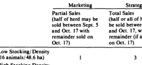
Four cases were modeled with 2 selling strategies and 2 stocking densities (Table 1). In cases I and 2, half of the herd may be sold between 5 September and 17 October, with the remainder sold on 17 October 17 (traditional selling date). Cases 3 and 4 provide that half or all of the herd may be sold between September 5 and October 17, with the remainder of the cattle (if any) sold on October 17. The stocking density was 0.33 animals/ha (16 year- lings in a 48.6 ha pasture) for cases I and 3, and 0.49 animals/ ha (24 yearlings in a 48.6 ha pasture) for cases 2 and 4. The selected pasture size was not typical of yearling operations, but it could easily be adjusted to the pasture size of an existing ranch. Empirical equations for vegetation and animal growth were determined by regression analysis, and assembled into the DP model. A general- ized DP package (Labadie et al. 1982) was used to maximize net present value for the 4 cases previously described.

Table 1. The four cases modeled under different stocking densities and marketing str8tegiea.

Marketing Strategy

Partial Sales Total Sales

(half of herd may be (half or all of herd may sold between Sept. 5 be sold between Sept. 5 and Oct. 17 with and Oct. 17, with remainder sold on remainder (if any), sold Oct. 17) on Oct. 17)

Low Stocking/Density

(I6 animals/48.6 ha) I 3

High Stocking Density

(24 animals/48.6 ha) 2 4

The Dynamic Optimization Model

The model used here was dynamic in the sense that it optimized the sequence of decisions throughout the grazing season, in con- trast to static models that optimize over the entire grazing season. The dynamic optimization model had 3 variables: (I) standing crop of vegetation (SCV) ranging from 400 to 620 kg/ ha with 20-kg/ha intervals; (2) average animal weight (AWT) ranging from 235 to 350 kg with 5-kg intervals; and (3) number of animals per area (D) with 2 discrete values, 24 or 12 animals per 48.6 ha (high stocking density) and 16 or 8 animals per 48.6 ha (low stocking density). These discrete numbers are related to zero and 50% herd sales. Each of these state variables is related to 3 fundamental processes: forage growth, animal growth, and change in number of animals in the operation. Eleven stages were designated from late May to mid October. The beginning of stage 11 was only considered as the outcome of stage 10. A stage (subscript t) was defined as a 14-15 day period. At the beginning of that period, a decision (control u, defined below) was made and applied to the rest of that period (Fig. 1). Changes in number of animals depended upon the selling alternatives selected during the grazing season; these alternatives were considered in concert with supplementation alternatives. The DP recursive relation can be written as follows:

Ft(AWTt,SCVt,Dt) = Max ((Pit Yh. - TOTSUPPt P2, - VLABORJ u _{+ BFt+l (AWTttl.SCVttlDt+l) - FOt) (1)} where Pit and P2r were the steer prices in the Omaha market (USDA 1984)and cottonseed meal (USDA 1985)at stage t, respec- tively; TOTSUPPt was the weight of cottonseed meal fed to cattle during stage t (according to Bement 1970); VLABORtwas the cost of veterinary and labor expenses for stage t. This value was calcu- lated as 30 cents animal/day without supplementation, and 35 cents with supplementation*. Fixed outlay (FOt) was the initial cash paid for the steers (USDA 1984), this amount was zero for all stages other than 11 (beginning of the computational procedure). Fixed costs, such as land, were not considered. Ft was the maxi- mum net present value at stage t and Ft+l was the maximum accumulated net present value from previous stages where B was the discount factor based on 14% nominal annual interest rate.

Maximization in (1) utilized 5 different decisions (u) at each stage t:

When: u=l all livestock were marketed, u=2 livestock were supplemented,

u=3 the initial grazing scheme was maintained,

u=4 50% of livestock were marketed and the remaining animals were supplemented, and

u=5 5% of livestock were marketed and the remaining animals were not supplemented.

The quantity of livestock sold at stage t (Y&S

IC. Kerry Gee. United States Department of Agriculture, Economic Research Service, Department of Agricultural and Resource Economics, Colorado State University (personal communication).

following relation:

Y,,” = f (AWTtiD,,u) (2)

where Yt,” depended on number of animals per pasture (DS, the average weight (AWTS, and the decision u.

Average animal weight at stage t (AWTt) in equation 1 was defined by the following equation:

AWTt = AWTt-I + ADGt NODAYSt. (3)

Average animal weight in stage t depended on the average animal weight in the previous stage (AWTt-1) plus net animal growth (the product of the average daily gain at stage t (ADGS times the number of days (NODAYSS for that stage).

Average daily gain (kg per animal per day) at stage t was calcu- lated with the following equation:

ADG, = Z (-.895 + 902 RLNz+wr). (4)

Where Z was an adjusting factor for grazing conditions (dis- cussed below), and the relative limiting nutrient (Senft et al. 1984) for a specific weight (RLN,&r) was defined by the following expression:

RLNAw = Min (CPINT/ CP,, DEINT/ DEIll) . (5)

The minimum of 2 ratios, crude protein intake (CPINT) to crude protein for daily maintenance (CPS and digestible energy intake (DEINT) to digestible energy for daily maintenance (DEm). Daily intake and maintenance requirements (crude protein and digestible energy) for 250 to 400 kg steers gaining 0 to I kg of weight per day (NRC 1976) were used to estimate the linear function in paren- theses of equation 4. This equation was highly significant (Rzz.99, p<Ol) in predicting average daily gains for steers under feedlot

conditions.

Under grazing conditions, average forage intake (AVEINTt) was estimated with Conrad’s et al. (1964) equation multiplied by a linear decreasing function:

AVEINTt = (.0107 AWTJ (I-DMD)) G(AWTS. (6)

Where DMD was in-vitro dry matter digestibility of forage. According to Bourdon (1983), Conrad’s equation (first term in parentheses) underestimated the ratio fecal dry matter to live weight (.0107) in growing steers. To compensate for underestima- tion, G(AWTS was a linear decreasing function from 1.1 to 1.0, representing 10% extra forage intake for 235 kg steers and 0% for animals weighing 340 kg or heavier. Forage crude protein and in-vitro dry matter digestibility (Table 2) plus crude protein and

Table 2. Percentage of crude protein (CP) aad in-vitro dry matter dlgeati- bility (DMD) for tke gmzing aeason at CPER.

Period Stage CP DMD

5130 6/12 I 12.9 59.1

6113 6126 2 12.0 61.1

6127 7110 3 IO.8 59.5

7/ll 7124 4 9.8 56.9

7125 817 5 9.4 56.7

818 E/21 6 9.1 55.2

a/22 914 7 8.1 53.2

915 9119 8 7.1 51.1

9120 IO/3 9 6.8 51.7

IO/4 IO/ I7 10 6.5 52.2

Interpolated figures from monthly data reported in Dean and Rice (1975). Senft (1983), Uresk and Sims (1975) and Vavra et al. (1973).

Beginning

horizon.

of planning

May 30.

Forage utilizatibn is evaluated

Fig. 1. Temporalframework of the planning horizon and the sequence of stages in the DP.

dry matter digestibility of supplement (if provided), were used to calculate CPINT and DEINT. Daily maintenance requirements for crude protein and digestible energy were calculated with equa- tions provided in NRC (1976) to compute RLN*m. Subsequently, ADGtwas calculated only with the term in parentheses of equation 4. This equation underestimated average daily gains (without sup- plementation) reported by Bement (1968), Dyck and Bement (1971, 1972) and Senft (1983) at CPER. As a result, the constant Zz1.42 in equation 4 was an adjusting factor to grazing conditions at CPER. This constant was larger than 1, suggesting that steers with equal RLN value will gain more by grazing over feedlot conditions. The value of this constant can be explained by 2 arguments: (1) Animal selectivity affects CPINT and DEINT, and equation 6 did not imply that grazing animals select forage with higher quality than average; (2) According to Denham and Spreen (1986), NRC (1976, 1984) overestimates maintenance require- ments and underestimates efficiency in utilizing metabolic energy under high forage diets.

Standing crop of vegetation at stage t (SCVt) in equation 1 was defined by the following equation:

SCVt = SCVH + ANPPt - TOTINTt ₍₇₎

where ANPPt was the aboveground net primary productivity per stage t (kg/ha). This was defined as follows:

ANPpt q 14.44 + 4.098 PPTt-, + 1.726 PPTt - .174 SCvbl ₍₈₎

(Rz = .67,p<.Ol). Aboveground net primary productivity depended on precipitation (mm)during the previous and current stage (PPTt-1 and PPTt, respectively), as well as standing crop of vegetation in the previous stage (SCVt-1). Equation 8 was determined with biweekly data from Bement (1968) and Dyck and Bement (1971, 1972). Total intake at stage t (TOTINT*) in kg/ ha was defined as:

TOTINTt = AVEINTt D, NODAY&, (9)

296

horizon.

17.

where AVEINTt is average forage intake (kg per day per animal), Average forage intake was limited to 80%~ of estimated AVEINTtif a forage reserve level was lower than 380 kg/ ha as a consequence of forage overutilization. This condition defined a step function that related a threshold value of standing crop to animal intake, this assumed condition was used in the absence of empirical data for this relationship. Therefore, AVEINTt was dependent on the decreasing forage quality (DMD in Table 2) and possible shortage of forage (below the forage reserve level). In the absence of empiri- cal relationships that relate stocking densities and forage quality dynamics, this model assumed that stocking density per se did not exacerbate the temporal decreasing trend in forage quality.

Density of animals at stage t (Dt) in equation 1 was defined by the following equation:

Dt = Dt-1 -DdYt.S , WV

where the number of animals per pasture at stage t (Dt) was equal to the density of animals in the previous stage (Dt-1) minus the number of animals sold in stage t (DdYt,)).

Results and Discussion

Cases 1 and 2 allowed partial sales at a given marketing date and utilized low and high stocking density, respectively. Optimal tra- jectories of the variables are described below.

Standing crop of vegetation followed similar trajectories for the 2 cases. During the first 3 stages there was a net increase in the standing crop (Fig. 2) corresponding to 97 mm of precipitation at CPER during that period (52% of the total rainfall during the grazing season). The standing crop of vegetation during the next 3 stages was stable while in the last 4 stages declined. The final standing crop of vegetation was 40 (low stocking density) and 20 (high stocking density) kg/ha above the initial 400 kg/ha at the beginning of the grazing season.

Under low stocking density, the number of animals per area during the first 9 stages was 16; at the beginning of stage 10 half of

::o

TIMi

stage1

Fig. 2. Optimal trajectories of the state variables under partial sales strategy.

the animals were sold and 8 were kept to be marketed at the beginning of stage Il. Animals per area under high stocking den- sity were kept at 24 during the first 8 stages and decreased to 12 during stages 9 and IO. This suggested that greater grazing pressure prompted the decision to reduce the pressure one stage sooner than in the case of low stocking density. In order to avoid reduced forage intake and decreased animal growth, the stocking density was adjusted, resulting in partial sales.

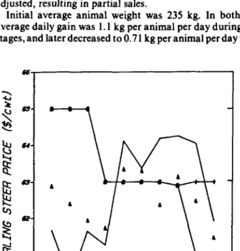
Initial average animal weight was 235 kg. In both cases the average daily gain was 1.1 kg per animal per day during the first 3 stages, and later decreased to 0.7 1 kg per animal per day for the rest

#*op + m?mwlN - a%4orace8 L mm*lcoe

Fig. 3. Yearling steer price and average daily gain with respect to time.

JOURNAL OF RANGE MANAGEMENT 40(4), July 1987

of the grazing season, resulting in a final weight of 350 kg at the beginning of stage 11. Supplementation was .provided during stages 9 and 10 in both cases, preventing average daily gains of only .36 kg per animal per day.

Steer prices ($/cwt) in 1984followed the trend of the last 4 years (USDA 1984), as shown in Figure 3. Declining livestock prices towards the end of the grazing season must be taken into consider- ation since they affect net revenue. Using a low stocking density, livestock were sold early not because of forage overutilization but because it was more profitable to sell at stage 10 than stage 11. This was an economic decision based on the principle that additional revenue of retaining livestock one more stage must be larger or equal to the additional costs associated to that stage. This decision rule applies for discrete cases such as the ones presented here (i.e., the changes in returns and costs are calculated between stages or periods of time, as opposed to infinitesimal changes). For example, the revenue of selling steers at the beginning of stage 9 was $467.02 (330 kg divided by .454 kg/ pound multiplied by $64.25 and divided by 100 pounds); similarly, the revenues for selling cattle at stages 10 and 11 were $479.54 and $477.35, respectively. Total variable costs without supplementation at the beginning of stage 9 were $33.90, while total variable costs with supplementation the beginning of stages 10 and 11 were $39.36 and $44.44, respectively.

The difference between the change in revenues and the change in total variable costs between stages 9 and 10 was $7.06 (($479.54- 467.02)-($39.36$33.90)). The analogous difference between stages 10 and 11 was -57.27 (($477.35-$479.54)-(%44.44-$39.36)). At the beginning of stage 9 it was decided to retain the steers until stage 10 with $7.06 net return per stage; in contrast, at the beginning of stage 10 it was decided to sell the animals to avoid $7.27 net loss per stage. The net present value per 48.6 ha pasture at the end of stage 10 was $1,437 and $2,160 for low and high stocking densities, respectively (Table 3).

Table 3. Net present value (S)l per 48.6 ha pasture at CPER under different marketing stategka and stocking densities.

Difference Marketing Strategy _{Between Total}

Partial Sales Total Sales and Partial Sales2

Low 1437 1529

Stocking Density (Sf%,

High 2160 2293

Stocking Density (3?%)

‘These calculations did not consider rent for land. depreciation of machinery or land investments.

‘The values in parentheses art the percent differences between total and partial s&S strategies with respect to total sale strategy.

Total Sales Marketing Strategy

Cases 3 (low stocking density) and 4 (high stocking density) allowed all of the animals to be sold at a given marketing date. As in the cases with partial sales strategy, SCV had a similar trend for both stocking densities. Under high stocking density, the SCV at the beginning of stage 10 was 400 kg/ha, equal to the initial SCV (Fig. 4). Under this marketing strategy, the forage resource was utilized close to the threshold level of 380 kg/ha. The number of animals per area was constant until all animals were sold at the end of stage 9 for the 2 stocking densities.

Initial animal weight was 235 kg. Under both stocking densities, animal growth was 1.1 kg per animal per day during the first 3 stages, decreasing to 0.71 kg per animal per day in the remaining stages. Supplementation took place in stage 9, and final weight was 340 kg at the beginning of stage 10.

Steer sales at the beginning of stage 10 were determined by the

6W

,i , . , . , _ , _ , .

J 9 9 7 9

TIME

(beginning

of stage)

SCV - St&%jJng crop of veg6trtJm 0 - Number of mJm6Js p6r we6 SD - StockJng density

F D IOU iv ___*__.

Fig. 4. i&lima1 rrajecrories of rhe slate variables under roral sales srrategy.

declining prices toward the end of the grazing season (Fig. 3), a similar situation to that under partial sales strategy and low stock- ing density. The net present value per 48.6 ha pasture at the beginning of stage 10 was $1,529 and $2,293 for low and high stocking densities, respectively (Table 3).

The difference in the net present value per pasture between total and partial sales strategies was larger for high stocking densities ($87=2,293-$2,160) than the difference in the net present value per pasture between total and partial sales strategies for low stocking densities ($58=%1,529-$1,437). These differences with respect to the net present values of the total marketing strategies were 3.8% in both stocking densities (Table 3). This percentage was a net return loss related to the retention of 5% of the herd at the end of stage 10 under the partial sales strategy.

Conclusions

The combination of decreasing yearling steer prices and declin- ing forage quality towards the end of the grazing season dictated early sales in spite of the possibility,of livestock growth. Supple- mentation offset the trend in decreasing average daily gain toward

the end of the grazing season. It was a selected control as long as gain in revenue compensated the increased total variable costs of retaining steers another stage.

Under high stocking density and partial sales strategy, early sale regulated end-of-season standing crop. Under low stocking density and partial sales strategy, early sale minimized net return losses for those animals that had to be sold at the traditional marketing date. The total sales strategy favored sales of steers 2 weeks before traditional marketing under low and high stocking densities. In all cases, except under high stocking density and partial sales strategy, decreasing steer prices determined the early sale of cattle. Net present values per pasture were slightly larger for the total sales strategy than the partial sales strategy using both low and high stocking densities.

298

Literature Cited

Bartlett,

Bement, R.E. 1968. Herbage growth rate and forage quality on shortgrass range. Ph.D. Diss. Colorado State University.

Bement, R.E. 1970. Fall gains of steers fed cottonseed cake on shortgrass

range. J. Range Manage. 23: 199-201.

Bourdon, R.M. 1983. Simulated effects of genotype and management on beef production efficiency. Ph.D. Diss. Colorado State University.

Burt, O.R. 1971. A dynamic economic model of pasture and range invest- ments. Amer. J. Agr. Econ. 53:197-205.

Conrad, H.R., A.D. Pratt, 8nd J.W. Hibbis. 1964. Regulation of feed intake in dairy cows. I. Change in the importance of physical and physiological factors with increasing digestibility. J. Dairy Sci. 4754-62. Dun, R.E. and R.W. Rice. 1975. Energy and nitrogen flow through cattle

on the shortgrass prairie. Grassland Biome. U.S. internat. Biol. Pro- gram. Tech. Rep. No. 293.

Denham, S.C., and T.H. Spreen. 1986. Introduction to simulation of beef cattle production. p. 39-62.1n:T.H. Spreenand D.H. Laughlin. Simula- tion of beef cattle production systems and its use in economic analysis. Westview Press, Boulder, Colo.

Dyck, G.W., and R.E. Bement. 1971. Herbage growth rate, forage intake and forage quality in 1970 on heavily and lightly grazed blue grama pastures. Grassland Biome. U.S. Internat. Biol. Program. Tech. Rep. No. 94.

Dyck, G.W., end R.E. Bement. 1972. Herbage growth rate, forage intake and forage quality in 1971 on heavily and lightly grazed blue grama pastures. Grassland Biome. U.S. Internat. Biol. Program. Tech. Rep. No. 182.

Fisher, I.H. 1985. Derivation of optimal stocking policies for grazing in arid regions. I. Methodology. Appl. Math. Comp. 17: I-35.

Hunter, D.H., E.T. Bartlett, and D.A. Jameson. 1976. Optimum forage allocation throughchance-constrained programming. Ecological Model- ling 2:91-99.

Kiippie, GE., and D.F. Costello. 1960. Vegetation and cattle responses to different intensities of grazing on shortgrass ranges on the Central Plains. USDA Tech. Bull. No. 1216.

Labrdie, J.W., J.M. Sheffer, and D.G. Fontane. 1982. CSUDP general purpose dynamic programming code. Dep. Civil Engineering, Colorado State Univ.

National Research Council (NRC). 1976. Nutrient requirements for beef

cattle. Nat. Acad. Sci. Washington, D.C.

National Research Council. 1984. Nutrient requirements for beef cattle. Nat. Acad. Sci. Washington, D.C.

Propoi, A. 1979. Dynamic linear programming models for livestock farms. Behavioral Sci. 24:200-207.

Sala, O.E., W.K. Lauenrotb, W.J. Parton, and M.J. Triica. 1981. Water status of soil and vegetation in a shortgrass steppe. Oecologia 48:327-33 1. Senft, R.L. 1983. The redistribution of nitrogen by cattle. Ph.D. Diss.

Colorado State Univ.

S&t, R.L., M.A. Stiiiweii,end L.R. Rittenhouse. 1984. Seasonal changes in nitrogen and energy budgets of cattle range. Amer. Sot. Anim. Sci. West. Sect. Proc. 35:2C&203.

Sharp, W.C. 1967. A dynamic programming model for evaluating invest- ments in mesquite control and alternative beef cattle systems. Texas A&M Univ. Texas Agr. Exp. Sta. Tech. Monogr. 4 (September).

Toft, H.I., and P.W. O’Hanion. 1979. A dynamic programming model for on-farm decision making in a drought. Rev. Market. and Agr. Econ. 47:5-16.

Trspp, J.N., and O.L. Walker. 1986. Biological simulation and its role in economic analysis. p. 13-37.In:T.H. Spreen and D.H. Laughlin (eds.), Simulation of beef cattle production systems and its use in economic analysis. Westview Press. Boulder, Colo.

Uresk, D.W., and P.L. Sims. 1975. Influence of grazing on crude protein content of blue grama. J. Range Manage. 28:370-371.

U.S. Depertment of Agriculture. 1984. Market news weekly summary and statistics. Livestock division. Agr. Marketing Serv. Washington, D.C. Vol. 49-52.

U.S. Department of Agriculture. 1985. Feed outlook situation report. Fds. 294-296.

Vavra, M., R.W. Rice, and R.E. Bement. 1973. Chemical composition of the diet intake, and gain of yearling cattle on different grazing intensities. J. Anim. Sci. 36:441-444.

Van Pooiien, H.W., and P. Lang. 1986. Analyzing the effect of changing feed-beef price relationships on beef production on management strate- gies in Hawaii: a dynamic programming approach. West J. Agr. Econ.

11:106-114.