An Environment for Developing Incremental Learning Applications for Data Streams

Scholarship@Western

Scholarship@Western

Electronic Thesis and Dissertation Repository

11-27-2019 10:30 AM

An Environment for Developing Incremental Learning Applications

An Environment for Developing Incremental Learning Applications

for Data Streams

for Data Streams

Farzin Sarvaramini

The University of Western Ontario

Supervisor Bauer, Michael A.

The University of Western Ontario Graduate Program in Computer Science

A thesis submitted in partial fulfillment of the requirements for the degree in Master of Science © Farzin Sarvaramini 2019

Follow this and additional works at: https://ir.lib.uwo.ca/etd

Part of the Artificial Intelligence and Robotics Commons

Recommended Citation Recommended Citation

Sarvaramini, Farzin, "An Environment for Developing Incremental Learning Applications for Data Streams" (2019). Electronic Thesis and Dissertation Repository. 6662.

https://ir.lib.uwo.ca/etd/6662

This Dissertation/Thesis is brought to you for free and open access by Scholarship@Western. It has been accepted for inclusion in Electronic Thesis and Dissertation Repository by an authorized administrator of

ii

Abstract

Smart cities look to leverage technology, particularly sensors, and software to provide

improved services for its citizenry and enhanced operational efficiencies. Cities look to

develop applications that can process data from sensors and other sources to gain insights

into operation, enable them to improve operations and inform city leadership. Such

applications often need to process streams of data from sensors or other sources to provide

city staff with insights into city operations. However, cities are faced with limited budgets

and limited staff. The development of applications by third parties can be extremely

expensive. One alternative is to identify tools for software development that city staff can

use – where the development tools can simplify the development process.

This research addresses this challenge by looking at a graphical flow-based programming

framework, Node-RED, as the foundation for a flexible application development

environment that can accelerate and simplify the development of applications of interest to

smart cities. Node-RED presents a visual programming framework composed of nodes and

data flows. We look at extending Node-RED to incorporate nodes that hide the complexity of

developing incremental machine learning applications by providing relatively simple and

easy to use graphical interfaces. Nodes for a variety of learning methods are introduced and

used for real-time analysis of data streams. Nodes providing different metrics have also been

designed to enable the application developer to evaluate the trained models.

Keywords

iii

Summary for Lay Audience

iv

Acknowledgments

v

Table of Contents

Abstract ... ii

Summary for Lay Audience ... iii

Acknowledgments... iv

Table of Contents ... v

List of Figures ... vii

Introduction ... 1

Literature Review ... 4

2.1 IoT Platforms ... 4

2.2 Real-Time analysis of IoT data ... 7

2.3 Incremental learning ... 8

Approach ... 11

3.1 Node-RED... 11

3.1.1 Node-RED’s editor components ... 12

3.1.2 Node-RED programming model ... 20

3.1.3 Building a node in Node-RED ... 22

3.1.4 Deployment of a Node-RED application ... 25

3.2 Incremental learning with Creme... 26

3.3 Building incremental learning nodes for Node-RED ... 27

3.3.1 Training ... 27

3.3.2 Metrics ... 30

3.3.3 Prediction and Evaluation ... 32

3.3.4 Utility Nodes ... 32

Experiments and Results ... 33

vi

4.2 Linear regression ... 33

4.3 Binary Classification ... 41

4.4 Multiclass Classification ... 42

4.5 Clustering ... 47

4.6 Summary ... 50

Conclusion ... 51

5.1 Summary ... 51

5.2 Future Work ... 51

References ... 53

Curriculum Vitae ... 57

vii

List of Figures

Figure 1: IoTLink abstraction layers’ metamodel. ... 6

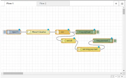
Figure 2: An example of a flow in Node-RED’s browser-based editor. ... 12

Figure 3: Node-RED’s editor components [19]. ... 13

Figure 4: Node-RED’s palette. ... 14

Figure 5: Node-RED’s workspace. ... 14

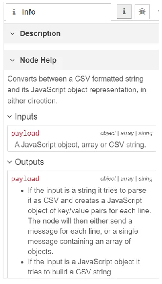
Figure 6: Information sidebar for the CSV node. ... 15

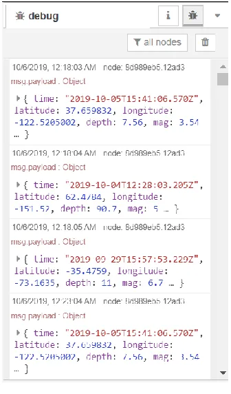
Figure 7: Debug message sidebar. ... 16

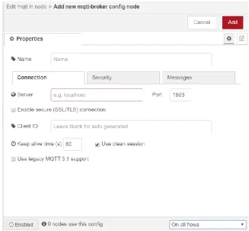
Figure 8: configuration node for the node MQTT. ... 17

Figure 9: Context panel ... 18

Figure 10: Node-RED’s palette manager. ... 19

Figure 11: properties of a CSV node. ... 20

Figure 12: The HTML file of a node called “lower-case” ... 23

Figure 13: Javascript code of an example node called “lower-case” ... 24

Figure 14: JSON file for the lower-case node. ... 25

Figure 15: The flow for publishing the current timestamp ... 26

Figure 16: The messages received by Kafka consumer ... 26

Figure 17: Example of Linear Regression’s node properties... 28

Figure 18: Linear regression training flow. ... 34

viii

Figure 20: Kafka object message with topic LR. ... 35

Figure 21: Parameters of the “set msg.payload” node. ... 35

Figure 22: The output of the “set msg.payload” node ... 36

Figure 23: Parameters of the “json” node. ... 36

Figure 24: Output of the “json” node. ... 37

Figure 25: Parameters of the “limit” node. ... 37

Figure 26: Parameters of the “Standard Scaler” node ... 38

Figure 27: The output of the “Standard Scaler” node. ... 38

Figure 28: Parameters of the “Linear Regression” node ... 39

Figure 29: Output of the “Linear Regression” node for a specific training instance. ... 39

Figure 30: The parameters of the “Regression Metric” node. ... 40

Figure 31: The output of the “Regression Metric” node. ... 40

Figure 32: MAE of the linear regression model ... 41

Figure 33: The flow of logistic regression training. ... 42

Figure 34: Accuracy of the logistic regression model. ... 42

Figure 35: Flow of training with multinomial regression. ... 43

Figure 36: Accuracy of the multinomial regression model ... 44

Figure 37: Flow of the one-vs-rest classification. ... 44

Figure 38: accuracy of the one-vs-rest classification. ... 45

ix

Figure 40: accuracy of the decision tree model. ... 46

Figure 41: Flow of the Gaussian naive Bayes classification. ... 46

Figure 42: accuracy of the Gaussian naive Bayes classification. ... 47

Figure 43: The generated dataset for clustering. ... 48

Figure 44: flow the clustering with KMeans. ... 48

Figure 45: Labeled instances by KMeans. ... 49

Figure 46: Result of typical batch KMeans ... 49

Chapter 1

Introduction

The main purpose of the internet of things (IoT) is connecting physical objects to the

Internet. IoT helps physical objects to be able to sense, send and receive messages,

perform computations and communicate with other physical objects through the Internet

to achieve an objective [1]. IoT applications have been used in a variety of domains like

enterprises, transportation, healthcare, communication, environment, and smart city.

Being able to connect objects creates the power of decision making and control which

results in huge benefits in many domains. Industries and governments are also investing a

considerable amount of money in IoT. According to Castillo and Thierer [2], by 2025, the

value of IoT technologies will be anywhere from $2.7 trillion to $14.4 trillion.

The continuous growth of IoT in every aspect of our lives has created the need to

develop, control and maintain IoT applications. However, creating IoT applications has

its own challenges. Heterogeneity of sensors, various protocols of communication, data

management and developing user-friendly graphical interfaces for monitoring of data are

some of the challenges of IoT development. These challenges are particularly significant

in the emergence of smart cities. Cities have limited funding and limited staff for

developing and maintaining applications. These difficulties make the development hard

and delay the progress of IoT applications in smart cities. In order to make this process

easier, we need platforms that can provide abstractions for the different layers of the

development so that people with different technical knowledge are able to meet their

needs by creating their own applications.

In order to be able to take advantage of the large amounts of data that is being produced

by different sensors, platforms need to provide tools for data analysis. Machine learning

is being used in many IoT applications, like in smart cities, to turn data into value and

make decisions that help the system perform more efficiently and more effectively. The

being used to predict electricity load [3], estimate solid waste generation [4], controlling

available parking slots [5] and many other applications.

In an IoT application sensors are continuously sensing their environment, producing data

and sending them to a system, a server or an edge processor, for storage, analysis, and

further distribution. In some applications, it is critical to make real-time decisions and be

reflective of the latest changes in the data. Most of the existing IoT platforms have

provided typical methods of machine learning that are only able to train on large batches

of data and usually require an expert to develop such applications. These models are

typically developed off-line. An alternative is to consider learning on streams of data.

The method of learning that can train and adjust the model on continuous streams of data

is called online machine learning or incremental machine learning.

Node-RED is a web-based visual programming tool that was first created by IBM for the

rapid development of IoT applications. Node-RED has a flow-based programming model

and connects data sources by “wiring” them together. Node-RED provides a rich set of

tools for application development and it is designed in a way that people with different

programming backgrounds can utilize its features to develop a data-intensive application.

Node-RED’s active community of developers has built tools for machine learning that

can be easily added to Node-RED. However, all the existing training methods are typical

machine learning algorithms that need the whole data (or large quantities of data) for

training. In our work, we look at the feasibility of building a set of tools for Node-RED

that enables users to have access to online machine learning methods and data

preprocessing functions that are specifically designed for online machine learning

settings.

The main contribution of this thesis is an environment for developing incremental

learning solutions for data streams. This environment contains methods for training

models, evaluating the models, and data preprocessing nodes. The environment has a

user-friendly graphical interface that facilitates the development process which enables

This thesis is structured as follows. In Chapter 2, we will look at a number of existing

tools that are trying to facilitate the development of IoT applications and discuss their

approaches for data analysis. Also, in this chapter, methods of incremental machine

learning will be introduced and compared with the batch machine learning. In Chapter 3,

we will explain Node-RED and the advantages that it offers for building IoT applications.

Then we discuss our contributions to Node-RED that enable developing incremental

machine learning solutions in simple steps. In Chapter 4, the provided approaches will be

evaluated using various datasets and we will walk through the steps for building an

incremental learning model using Node-RED. In Chapter 5, we provide a summary of

Chapter 2

Literature Review

IoT applications are now being used in many domains from medical and healthcare to

smart cities and agriculture. The advent of communication technologies like 5G is also

going to accelerate the growth of the number of devices that are connected to the Internet.

This raises the necessity of having software platforms that make the development of IoT

applications faster and easier. In this chapter, a number of IoT platforms, as well as their

efforts for data stream analysis, will be discussed.

2.1

IoT Platforms

In order to develop a platform for IoT development, some requirements should be

satisfied. Since IoT has a large number of applications, large amounts of users’ data is

transferred between various sources. Hence, there should be mechanisms to secure such

an environment. IoT applications are being used in areas that need their systems to be as

deterministic and real-time as possible. So IoT platform developers need to make sure to

design systems that can work in real-time environments. IoT applications are needed to

perform their tasks with the minimum help of humans so an important characteristic of an

IoT platform is to enable building applications that are intelligent enough to work without

human intervention.

The authors of the IoT framework IoTSuite [6] have designed and implemented a set of

tools to make IoT development easier. They have tried to provide tools for different

stages of developing an IoT application. Their first tool is an editor that lets the designers

write high-level code that specifies the architecture of the application and deployment

configurations. They provide a compiler that translates the high-level code to parser files.

IoTSuite has a Mapper component that converts the high-level computational services

like deployment specifications and architecture specifications into standardized data

structures. Decision mappers use these data structures to create mapping files that are

responsible to decide where each computational service will be deployed among the set

collects all the generated codes in different stages of parsing and creates packages that

contain device-specific codes that prepare them to be deployed on the devices. Finally,

the last tool is the Running system which is responsible to execute the codes on multiple

devices in a distributed way. Although IoTSuite has provided a complete set of tools for

IoT development, its high-level programming language is quite difficult to understand for

people with a limited programming background.

RapIoT [7] is a software toolkit that tries to take care of the low-level details of IoT

development so a developer can easily focus on application development. RapIoT helps

non-experts to design an IoT prototype quickly by providing a set of primitives that are

common among all IoT devices, so the user does not need to know any device-specific

details. The architecture of RapIoT consists of three tools. The first tool is RapEmbedded

that is an Arduino library to let developers define primitives for a sensor or device. An

example of a primitive could be the location and the level of pollution for an air quality

sensor. The second tool of RapIoT is RapMoblie that is a mobile app that acts as a

gateway to gather the data from installed devices and communicate with the application

that is on the cloud. The last tool is RapCloud that provides a set of APIs that lets

developers create applications and deploy them in the cloud. The mobile app retrieves the

primitives from the devices and sends them to the cloud. The app in the cloud performs

the needed operations and sends back the results to the mobile app. The need to have

access to a smartphone to be able to control the IoT devices and monitor the results has

made RapIoT hard to use in areas like smart cities that need better ways of interacting

with devices. However, it could be a very great choice for prototyping small IoT

applications in areas like smart homes.

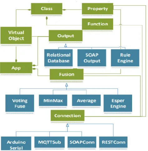
IoTLink [8] is another platform that aims to provide a set of tools that abstracts the

complexities of implementing an IoT application. There are four layers in the platform.

The first layer provides a high level and unified representation of connections between

different physical sensors. The second layer stands on top of sensor readings to collect

and aggregate the different sensors’ values and performs the required preprocessing. The

third layer abstracts the objects or “things” with their attributes. The fourth layer prepares

interfaces. Figure 1 depicts the aforementioned layers and their specific components in

IoTLink’s metamodel. IoTLink provides applications that are platform-independent, and

they can be transferred into a specific platform like Java. However, one disadvantage of

IoTLink over other platforms is the lack of a solution for the deployment of the

developed applications.

Figure 1: IoTLink abstraction layers’ metamodel.

Another platform is DataTweet [9] where the goal of its designers is to develop a

platform that eases the development of an IoT application. This platform has two main

entities. The first entity is application logic and the second one is common service entity

(CSE). The application logic is the part of the platform that IoT stakeholders interact

with. They use it to design user interfaces and implement the logic of the application.

The CSE takes care of common tasks among all IoT applications. Some of these common

procedures provide modules that enable using popular IoT protocols like HTTP and

MQTT. The other common services provided are the registration of new applications and

devices, device configuration management, data processing, and security. The CSE

provides abstractions in the lower IoT environment that helps the developers to focus on

2.2

Real-Time analysis of IoT data

In IoT, data from heterogeneous sources are often streaming data to servers, and an IoT

platform must be able to integrate these streams of data and provide tools for the

discovery of knowledge and analysis of data. The large scale of the data and the dynamic

environment of information are some of the challenges of real-time analysis of the data

streams.

One of the efforts for analyzing the streams of data is complex event processing (CEP)

[10]. CEP is a kind of stream processing system that performs queries on data without

any need to store the data. After defining patterns for the CEP engine, it is capable of

finding and matching those patterns in the continuous stream of data. CEP has a wide

range of applications in areas like business activity monitoring, sensor networks and

market data [11]. Esper [12] is a popular compiler and runtime environment for CEP that

is available for Java and .NET.

Other open-source frameworks that enable analysis on streams of data include S4 [13],

Apache Storm [14] and Apache Spark [15]. S4 [13] is a stream processing engine that has

inspired by MapReduce to build a distributed platform. S4 uses Hadoop in order to have a

MapReduce model for its engine. Using MapReduce helps to parallelize the tasks and run

them on a cluster of nodes. A problem with S4 is that the engine does not perform the

load balancing in the cluster automatically.

Apache Storm [14] is a real-time distributed stream processing engine that is able to

perform computations for large amounts of data. Since Storm is running on a cluster of

nodes, it is easily scalable by adding computational nodes. Running on a cluster of nodes

has made Storm applications fault-tolerant because any failure of a node will be handled

by other nodes in the cluster.

Currently, Apache Spark [15] is the most popular framework for big data analytics on

clusters. Spark introduced a resilient distributed dataset (RDD) which is the fundamental

data structure in Spark. RDDs are portioned across machines and if one of them fails

caching process in memory that makes Spark 10 to 100 times faster than the Hadoop in

some operations. Spark Streaming is a powerful library provided by Spark to process the

continuous streams of data with high throughput and fault tolerance. Although Spark has

interfaces for Scala, Python, Java, and R, it is still hard for people with low programming

skills to set up a Spark environment, write programs and benefit the advantages of Spark.

Although frameworks like Apache Spark, Apache Storm, and S4 offer various tools for

processing streams of data, they are not commonly used for other stages of IoT

application development. We prefer to use frameworks that, besides being able to process

streams of data, can integrate with heterogeneous data sources like MQTT, Kafka, TCP,

and REST and also have compatibility with IoT hardware like Arduino, Raspberry Pi, or

Android-based devices. In addition, platforms with visual programming interfaces make

the development and management of IoT applications much more accessible for IoT

application stakeholders.

2.3

Incremental learning

Nowadays, online users produce a huge amount of data every second from all around the

world. Every second, Google receives about 63 thousand search queries, around 6

thousand tweets are published on Twitter, almost 58 thousand videos are viewed on

YouTube, and around 280 transactions happen in Walmart. Companies analyze all these

generated data to make the best customer experience and increase their revenue. We also

have a similar situation in other areas, like smart cities. Sinaeepourfard, et al. [16] have

done a study in the city of Barcelona. They performed an estimation of the amount of

data that will be transmitted from sensors in the case of complete sensor coverage in the

city. They measured that each day around 8 GB of data will be transmitted from sensors.

This projection excludes the data that can be acquired from many other sources such as

mobile devices, surveillance cameras, or web services.

Machine learning methods are used to take advantage of this huge amount of data to get

insights about the behavior of the system. Classical machine learning approaches need

the whole batch of data to perform their training. These methods are not suitable for an

reflective of the new changes. With the arrival of new data, batch-learning methods need

to do the whole training process again and discard the former model which is

time-consuming and expensive regarding the computational resources.

In order to overcome the aforementioned problems, it is necessary to come up with ways

to train models on streams of data. This approach would let the model be up to date and

be representative of the latest changes in the data. Incremental or online learning is the

name that is assigned to these models. These models continuously integrate the data into

the model and spend less amount of time and space which makes them a suitable option

for real-time learning of large amounts of data. The definition of an incremental learning

algorithm is an algorithm that generates from a given stream of training data 𝑠1, 𝑠2, … 𝑠𝑡 a

sequence of models ℎ₁, ℎ₂, … ℎ_𝑡. The model ℎ_𝑖 only depends on ℎ_𝑖−1 and the recent p

examples 𝑠_𝑖, … 𝑠_𝑖−𝑝 with p being strictly limited.

According to the number p which is the number of instances that the model trains at

once, we can have either batch-incremental (p>1) or instance-incremental (p=1) learning.

In batch-incremental learning, every p example of data forms a batch and a classical

batch-learning method trains on the batch. Each training on each batch creates a model.

In this method, depending on the size of the window (p), we might end up having a large

number of models. Due to storage limitations, we may be forced to delete the older

models to have storage space for the new models. Then a voting method decides the

prediction based on all the results that have been achieved from all the existing models.

This method has significant disadvantages. First, the model needs to wait for a batch to

get full then it will start learning the new examples. The second problem happens when

parts of data that have been trained by the deleted models are somehow discarded from

our training process. Lastly, different voting schemes would have to be analyzed and

tested to find the one that best fits the problem.

On the other hand, instance-incremental methods train on every instance of data as it

arrives. These methods have solved some of the problems of batch-incremental methods,

however, they also have their own disadvantages. There are fewer algorithms available

be modified to train on instances. When learning on instances, at the beginning of the

training process, we cannot expect the model to have relatively accurate predictions and

depending on the data, the model needs to see a minimum number of instances before

starting to perform well.

Authors in [17] investigated a variety of methods for both batch-based and instance-based

methods of incremental learning for classification. They considered Support Vector

Machines, Decision Trees, and Logistic Regression for batch-incremental learning, and

Naive Bayes, Hoeffding Tree ensembles, and Stochastic Gradient Descent for instance

incremental learning. Then they carried out an extensive number of experiments by

training on both synthetic and real data. After comparing the results, they concluded that

instance-incremental methods perform as well as their equivalent batch-learning methods

Chapter 3

Approach

In this Chapter, I will walk through the proposed approach for building incremental

learning solutions that are easy to develop in an IoT environment. First, we discuss what

is Node-RED as a flow-based IoT tool and how its features have made the development

of IoT products much easier. Then Python’s incremental library Creme [18] will be

introduced. I will then explain how I used Creme to build a set of essential tools in

Node-RED, in order to solve a good range of machine learning problems for a data stream

environment.

3.1

Node-RED

Node-RED is an open-source tool for building Internet of Things (IoT) applications.

Node-RED is web-based and provides browser-based editor. It uses predefined blocks of

codes that are called nodes and wire these nodes together to perform a specific task

(Figure 2). There are three kinds of nodes: input nodes, processing nodes, and output

nodes. A set of connected nodes that carry out a specific task creates a ‘flow’. In addition

to IoT, Node-RED has been used in a wide range of applications which has resulted in a

large user base and an active developer community.

Node-RED was first created by IBM researchers Nick O’Leary and Dave Conway-Jones

and was released as an open-source project in 2013. IBM built Node-RED because they

were “looking for a way to simplify the process of hooking together systems and sensors

when building proof-of-concept technologies for customers”. Node-RED now is part of

Figure 2: An example of a flow in Node-RED’s browser-based editor.

The set of built-in nodes that Node-RED offers, which are accompanied by the visual

representation, have hidden the complexity of developing lots of tasks. Developers can

quickly put these nodes together to create flows. Node-RED has also an active developer

community that works on the core code or to design new nodes and flows to publish in

the Node-RED library. They keep developing new nodes and share them with other

developers. Node-RED also provides a function node that allows a user to write their own

functions using JavaScript. The ease of use that hides the programming details, the

growing set of predefined nodes by the developer community, and the flexibility in

defining new nodes and functions have made Node-RED a strong tool for the

development of IoT applications. In this project, Node-RED version 1.0.0 has been used.

3.1.1

Node-RED’s editor components

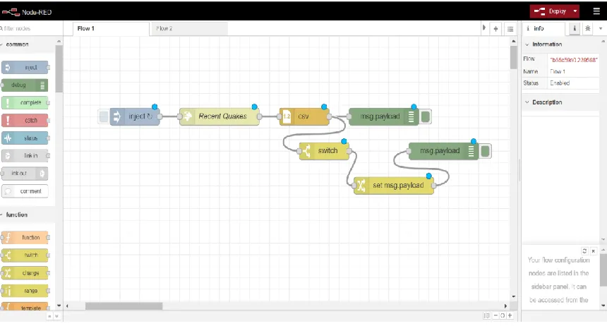
Node-RED’s editor has four components that are shown in Figure3.

3.1.1.1

Palette

Palette shows the list of the installed nodes in Node-RED (Figure 4) and it’s located on

set of default nodes that will be installed with Node-RED. In version 1.0.0 the existing

categories are common nodes, function, network, sequence, parser, and storage.

Figure 3: Node-RED’s editor components [19].

3.1.1.2

Workspace

Workspace is in the middle of the editor. Users drag the nodes to the workspace and wire

them together to create and design flows. A user can have multiple flows in one

Figure 4: Node-RED’s palette.

3.1.1.3

Sidebar

The sidebar is located at the right side of the editor and contains four sub-panels: node

information panel, debug panel, configuration panel and context panel. When a node is

selected, the node’s information bar shows the node’s help information. Figure 6 shows a

part of the information sidebar for the CSV node. It explains the functionality of the

node, inputs, and outputs.

The other panel in the sidebar is the debug message panel that is responsible for

displaying the logs in the flow. It shows messages that have passed through Node-RED’s

debug nodes. By default, the debug message displays all the debug nodes’ messages, but

it is possible to filter them to only see the messages of the selected nodes. Figure 7 shows

the debug sidebar displaying the messages that have been received by the debug node.

Figure 7: Debug message sidebar.

The configuration node allows the nodes to create and share a specific configuration to

other nodes. For instance, the “MQTT in” node can share the configurations for

connecting to the MQTT broker with the node “MQTT out” since they are both using the

same MQTT broker. Configurations are globally scoped by default which means they can

be used in different flows. Figure 8 shows the configuration node for the node “MQTT

Figure 8: configuration node for the node MQTT.

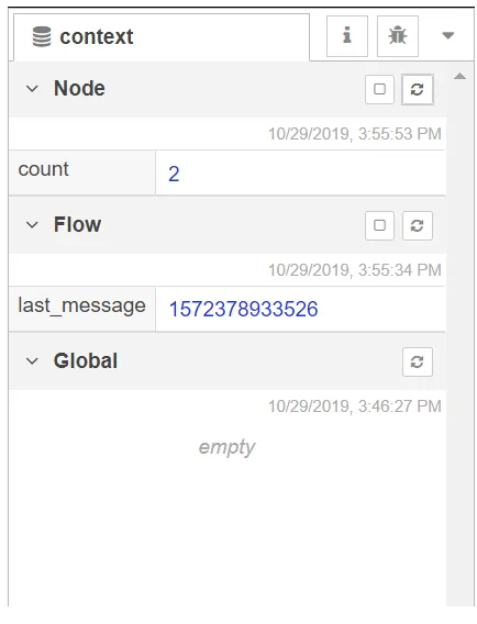
In Node-RED, messages are not the best place for storing variables because when a new

message arrives it will be replaced with the former message and we lose the former

message information. Node-RED has created context variables for storing information.

Every context variable has a scope. The scopes are node, flow and global. The node

scope means that only the node that has set the value of the context variable has access to

that variable. Flow scope means when a node puts value in a context variable, all the

nodes in the same flow have access to that context variable. And finally, the global scope

means all the nodes in all the flows have access to the context variable. Figure 9 pictures

the context panel of the sidebar. In the context panel, we can see the list of context

Figure 9: Context panel

The palette manager and the edit dialog are two other important components in

Node-RED that need to be explained.

3.1.1.4

Palette Manager

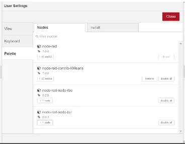
The other important section of the Node-RED’s editor is the palette manager (Figure 10)

that can be accessed by clicking the palette tab in the user settings. Under the nodes tab,

we can see the installed nodes. Users can disable or remove a specific node through this

window. The other tab is the install tab that gives the ability to search through the

repository of nodes in the Node-RED library and add them to the Node-RED’s local set

of nodes by installing them.

3.1.1.5

Edit Dialog

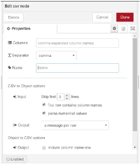
By double-clicking a node in the workspace, edit dialog will pop up. Edit dialog has three

• The Properties tab shows the features and parameters of a node that can be

changed by the developer. Figure 11 shows the properties of a CSV node.

• The Description tab allows the developer to write any explanation about the node.

This description will be displayed in the sidebar.

• The Appearance tab allows the developers to have small modifications in the appearance of a node like a node’s icon.

Figure 11: properties of a CSV node.

3.1.2

Node-RED programming model

A more detailed look at the Node-RED’s flow-based programming model will be

considered in this section. The main components such as messages, nodes, and flows will

be explained to get a better understanding of the Node-RED’s architecture.

3.1.2.1

Nodes

Nodes are small predefined functions that carry out a specific task. Just like functions,

they receive input, perform a process and then return the outputs. Each node can have at

most one input. An input to a node is a message that has been generated by another node.

In a node implementation, each node is made of two files. An HTML file that specifies

the appearance of a node such as its color, icon, name, node configurations and the

information window that explains the node and the parameters of the node. The other file

When the address of the Node-RED is accessed in the browser, the codes for each node

are loaded in the browser.

There are three types of nodes:

• Input nodes: These nodes initialize the start of a flow and generate the initial

message. An external stimulator like an HTTP request, a click by a user, or a TCP

message triggers the input node and causes the flow to start. Input nodes do not

have connecting points on the left side which means they cannot have inputs from

other nodes.

• Processing nodes: these nodes perform a specific task on each message. They

have a connecting dot at the left side of the node that allows them to get inputs

from other nodes. After receiving the message, they execute the function and

modify the message. Then the updated message will be passed to the node that is

connected to the connecting dot on the right side of the processing node. Some of

the built-in processing nodes can join, split, switch and change data. If Node-RED

does not have a processing node that someone is looking for, it is possible to

implement a custom processing node. The function node in Node-RED allows

implementing any function by writing a JavaScript code.

• Output nodes: These nodes send the final message outside the Node-RED flow either to the debug console, a device, or as a Kafka message it can send them to

the Kafka broker. Output nodes do not have connecting dots on their right side

which means they do not send messages to other nodes and they end a flow.

3.1.2.2

Messages

The information that passes through the nodes in Node-RED is called a “message”. A

message is simply a JavaScript object with some properties. The most important property

of a message is msg.payload that contains the data we are trying to pass from a node to

another node. The payload property can contain data of any type like string, Boolean,

number, JavaScript object, etc. The other property of a message is msg._msgid that can

property is msg.topic that allows assigning a topic to the message to increase the

readability and understanding the purpose of the message. Below we can see an example

of a message.

{

_msgid: '1db99c6d.e24664', topic: '',

payload: {} };

Node-RED does not restrain the users and let them add custom properties to their

message. Since msg.payload can get modified when a message passes through nodes, we

can use custom properties to pass specific data to a certain node.

3.1.2.3

Flows

A flow is a set of connected nodes that exchange messages to perform a specific task.

Under the hood, Node-RED stores flows as JavaScript objects that describe how the

nodes are connected and what each node configuration looks like.

3.1.3

Building a node in Node-RED

In order to define a new node, three files must be created. An HTML file that specifies

the node’s appearance, a JavaScript file that defines the functionality of a node, and a

JSON file that prepares a node to be installed with Node.JS package manager npm. Since

Python is used to take advantage of its capabilities in online machine learning, each node

usually has a Python file as well as the other three files. An overview of the structure of

each file will be presented in the following.

3.1.3.1

HTML file

The HTML file consists of three sections where each is inside a <script> tag. Figure 12 is

the HTML file for a node called “lower-case” that can show these sections. This node

converts all the characters of the message payload to lower case characters.

1. The first section registers a node in Node-RED’s list of local nodes. The default

values of a node’s parameters, the node’s icon, its color, and the category that it

2. The second segment which is defined under the type “text/x-red” with

“data-template-name” defines the node’s name and specifies the properties of the node

that can be edited by the users and their input type.

3. The help segment which is identified by assigning the “data-help-name” to the

node’s name, allows the developer to write a help description for the node to

explain any information about the node.

Figure 12: The HTML file of a node called “lower-case”

3.1.3.2

JavaScript file

The JavaScript file defines the logic and behavior of a node. Some of the main parts of

the JavaScript file are:

1. Constructor: it is responsible to create an instance of the node. It receives the

parameters that are set by the user in the edit dialog and assigns them to the

node’s instance.

2. Message listener: an event listener will be registered to hear the messages that are

In addition, we can listen to the errors that might happen during the process of

handling a message.

3. Sending a message: after processing the input message, the node can send a

message to the connected nodes.

Figure 13 shows the aforementioned sections in the Javascript file of the lower-case

node.

Figure 13: Javascript code of an example node called “lower-case”

3.1.3.3

Package.json file

Like any other module in NodeJS, in order to install a node, a package.json file is needed

to describe the module. Information like the list of nodes in the module, the given name

to the list of nodes, authors’ names, and the license are mentioned in this file. Figure 14

Figure 14: JSON file for the lower-case node.

3.1.4

Deployment of a Node-RED application

Since we are running Node-RED in the terminal, Node-RED is a child process of the

shell. This means that when we shut down the terminal, the Node-RED application will

be also terminated. In order to keep the Node-RED application running, we need to

detach the process from the terminal. We can use the screen command for detaching a

process from the terminal. The details of using this command for attaching and detaching

a process can be found in [20]. As an example, the flow shown in Figure 15 is an

application that publishes the current timestamp as a Kafka message. A python

application was also programmed to consume Kafka messages. After running the

application, I detached the Node-RED process from the terminal and closed the terminal.

We can even close the Node-RED editor in the browser and the application keeps

running. Figure 16 shows the messages received by the consumer while I had closed the

terminal and Node-RED editor. We might also consider deploying our application in a

remote machine. We can use a cloud-computing platform like Amazon Web Services for

hosting our application. Amazon EC2 provides virtual machines that can be rented and be

used to host our application. First, we need to install Node-RED in the remote virtual

machine. Then we need to use a process manager like PM2 [21] to run Node-RED on

Figure 15: The flow for publishing the current timestamp

Figure 16: The messages received by Kafka consumer

3.2

Incremental learning with Creme

Creme is an online machine learning library for Python. It is written with Python and the

style of APIs is inspired by Python’s machine learning library Scikit-learn [22]. Creme

can train on streams of data. In contrast to batch learning that needs to have access to the

entire data, Creme has been designed to train machine learning models by receiving one

instance of data at a time.

Creme provides different sets of tools for developing an online machine learning model

and they are continuously adding more features to their library. Binary and multi-class

classifiers, regressors, unsupervised clustering, ensemble learning, and tools for data

preprocessing and feature extraction are some of the main parts of their library.

For some operations like scaling the data, the model needs the whole data to compute the

mean and variance. However, receiving the data in a stream format creates the need for

called “running statistics” that compute an online version of operations like mean,

variance, entropy, correlation, etc. These functions are also used to build some of the

training methods. For instance, KMeans uses the running mean to update its centers and

clusters.

3.3

Building incremental learning nodes for Node-RED

Node-RED’s developer community has designed various machine learning nodes for

Node-RED, however, all the nodes are only designed for batch-oriented machine

learning. These methods usually store the whole data in a file and then train a model on

that data. IoT data is usually in the form of a stream so it is important to have learning

methods that can handle stream data and find the patterns in real-time. I used Python and

the Creme library to build a set of nodes for Node-RED that makes it possible to perform

online machine learning tasks in Node-RED.

A typical approach to train a machine learning model consists of preparing the data,

picking the right model, training, evaluating the results, and then using the trained model

to perform predictions on the new data. I have developed a set of nodes that are

considered essential tools for covering a normal range of machine learning problems,

including models for both supervised and unsupervised learning and different tasks such

as classification, regression, and clustering.

3.3.1

Training

Different nodes for training machine learning models have been implemented. Any

training node follows three steps after receiving an instance of the data. In the first step,

before training on the new data, the model predicts the target based on the existing

model. This gives us the opportunity to see how the model performs and to evaluate the

model at every single step. It helps us to monitor the progress of the model’s

performance from the very beginning of the training process. This way there is no need to

split some part of the data for validation because for any instance of the training data a

validation test happens. In the second step, the model trains on the data based on the true

Now different types of training models will be discussed.

3.3.1.1

Regression

Linear regression is a common approach for data analysis and building predictive models.

Developers need to specify some parameters of the model in the editor, otherwise, default

values will be assigned. One of the parameters is the optimization technique. Developers

can pick from AdaBound [23], AdaDelta [24], AdaGrad [25], Adam [26], Momentum

[27], NestrovMomentum [27], RMSProp [27], VanillaSGD [28], and FTRLProximal

[29]. Any of these optimizers have their own set of parameters that can be set. For

example, if we pick Adam, as we can see in Figure 17, the parameters that are needed for

Adam’s optimization will pop up. The other parameters that are needed for linear

regression are L2 regularization amount, address to save the model, and the target value’s

name.

3.3.1.2

Binary classification

Binary classification is a type of problem where the target can only have two possible

values. For this type of machine learning problem, a logistic regression node has been

implemented. The logistic regression node’s parameters are the path to store the model,

L2 regularization, name of the target index, and the optimization technique.

3.3.1.3

Multi-class classification

Machine learning problems where the target value has a range of more than two classes

are called multi-class classifications. This is a generalization of binary classification

problems. The first node that has been implemented to solve these problems is the

multinomial logistic regression which is a generalization of logistic regression for

multi-class multi-classification. The parameters of multinomial logistic regression are the same as

logistic regression.

The other classifier implemented is one-vs-rest classifier. This method assigns a binary

classifier for each class of the target value. For stream data, since we may not know the

number of classes in the beginning, the one-vs-rest classifier can be suitable because it

generates a classifier on the fly for each new class. The parameters are the same as

logistic regression since each of the independent binary classifiers is a logistic regression

classifier.

The third classifier is the decision tree classifier that is implemented based on the work of

Domingos et al. [30]. The parameters are patience, which is the timeout parameter

between split attempts [31], maximum tree depth, the minimum number of child samples,

confidence, and tie threshold. Those developers who do not have enough information

about the parameters can leave them blank so the default values would be assigned.

The last classifier for multi-class classification is Gaussian naive Bayes. This method

assigns a gaussian distribution for each class of the target. The parameters are model save

3.3.1.4

Unsupervised clustering

Unsupervised clustering refers to problems in machine learning where the aim is to

divide unlabeled data into clusters with similar features. For this purpose, a KMeans node

has been implemented. For KMeans the user needs to specify the number of clusters,

half-life, mu, and sigma. In incremental KMeans, each instance is assigned to the closest

cluster and then the center of the cluster will move toward the new instance. The half-life

parameter determines the amount that the center of the cluster will move toward the new

assigned instance. Mu and sigma are the mean and standard deviation of the normal

distribution that instantiates the cluster positions.

3.3.2

Metrics

Two metric nodes are designed for evaluating the results of the training nodes. After

every training node, a metric node can be used to compute the performance of the model.

Metric nodes need the predicted value and the true value as their inputs. A classification

metric node and a regression metric node have been implemented. Classification metric

node contains some of the popular metrics for classification problems. With the

classification metric node, a developer can pick any method from the options accuracy,

cross-entropy, macro F1, macro precision, macro recall, micro F1, micro precision, and

micro recall.

Accuracy is the percentage of the correct predictions. Cross-entropy is the other metric

that for a classification problem with 2 classes can be calculated as:

−(𝑦 log(𝑝) + (1 − 𝑦) log(1 − 𝑝)) .

Where y is the binary class of the target value (0 or 1), and p is the predicted probability

of the class.

F1, precision, and recall are also widely used for evaluating the results of a classification

problem. Below we can see how each of these metrics is calculated.

𝑃𝑟𝑒𝑐𝑖𝑠𝑖𝑜𝑛 = 𝑇𝑟𝑢𝑒 𝑃𝑜𝑠𝑖𝑡𝑖𝑣𝑒

𝑅𝑒𝑐𝑎𝑙𝑙 = 𝑇𝑟𝑢𝑒 𝑃𝑜𝑠𝑖𝑡𝑖𝑣𝑒

𝑇𝑟𝑢𝑒 𝑃𝑜𝑠𝑖𝑡𝑖𝑣𝑒 + 𝐹𝑎𝑙𝑠𝑒 𝑁𝑒𝑔𝑎𝑡𝑖𝑣𝑒

𝐹1 = 2 × 𝑃𝑟𝑒𝑐𝑖𝑠𝑖𝑜𝑛 ∗ 𝑅𝑒𝑐𝑎𝑙𝑙 𝑃𝑟𝑒𝑐𝑖𝑠𝑖𝑜𝑛 + 𝑅𝑒𝑐𝑎𝑙𝑙

The macro average of each of these metrics for a dataset with two classes is calculated as

below:

𝑀𝑎𝑐𝑟𝑜 𝑃𝑟𝑒𝑐𝑖𝑠𝑖𝑜𝑛 = 𝑃𝑟𝑒𝑐𝑖𝑠𝑖𝑜𝑛1 + 𝑃𝑟𝑒𝑐𝑖𝑠𝑖𝑜𝑛2 2

𝑀𝑎𝑐𝑟𝑜 𝑅𝑒𝑐𝑎𝑙𝑙 = 𝑅𝑒𝑐𝑎𝑙𝑙1 + 𝑅𝑒𝑐𝑎𝑙𝑙2 2

𝑀𝑎𝑐𝑟𝑜 𝐹1 = 2 × 𝑀𝑎𝑐𝑟𝑜 𝑃𝑟𝑒𝑐𝑖𝑠𝑖𝑜𝑛 ∗ 𝑀𝑎𝑐𝑟𝑜 𝑅𝑒𝑐𝑎𝑙𝑙 𝑀𝑎𝑐𝑟𝑜 𝑃𝑟𝑒𝑐𝑖𝑠𝑖𝑜𝑛 + 𝑀𝑎𝑐𝑟𝑜 𝑅𝑒𝑐𝑎𝑙𝑙

And we compute the micro averages of these metrics with the following equations:

𝑀𝑖𝑐𝑟𝑜 𝑃𝑟𝑒𝑐𝑖𝑠𝑖𝑜𝑛 = 𝑇𝑟𝑢𝑒 𝑃𝑜𝑠𝑖𝑡𝑖𝑣𝑒1 + 𝑇𝑟𝑢𝑒 𝑃𝑜𝑠𝑖𝑡𝑖𝑣𝑒 2

𝑇𝑟𝑢𝑒 𝑃𝑜𝑠𝑖𝑡𝑖𝑣𝑒1 + 𝐹𝑎𝑙𝑠𝑒 𝑃𝑜𝑠𝑖𝑡𝑖𝑣𝑒1 + 𝑇𝑟𝑢𝑒 𝑃𝑜𝑠𝑖𝑡𝑖𝑣𝑒2 + 𝐹𝑎𝑙𝑠𝑒 𝑃𝑜𝑠𝑖𝑡𝑖𝑣𝑒2

𝑀𝑖𝑐𝑟𝑜 𝑅𝑒𝑐𝑎𝑙𝑙 = 𝑇𝑟𝑢𝑒 𝑃𝑜𝑠𝑖𝑡𝑖𝑣𝑒1 + 𝑇𝑟𝑢𝑒 𝑃𝑜𝑠𝑖𝑡𝑖𝑣𝑒2

𝑇𝑟𝑢𝑒 𝑃𝑜𝑠𝑖𝑡𝑖𝑣𝑒1 + 𝐹𝑎𝑙𝑠𝑒 𝑁𝑒𝑔𝑎𝑡𝑖𝑣𝑒1 + 𝑇𝑟𝑢𝑒 𝑃𝑜𝑠𝑖𝑡𝑖𝑣𝑒2 + 𝐹𝑎𝑙𝑠𝑒 𝑁𝑒𝑔𝑎𝑡𝑖𝑣𝑒2

𝑀𝑖𝑐𝑟𝑜 𝐹1 = 2 × 𝑀𝑖𝑐𝑟𝑜 𝑃𝑟𝑒𝑐𝑖𝑠𝑖𝑜𝑛 ∗ 𝑀𝑖𝑐𝑟𝑜 𝑅𝑒𝑐𝑎𝑙𝑙 𝑀𝑖𝑐𝑟𝑜 𝑃𝑟𝑒𝑐𝑖𝑠𝑖𝑜𝑛 + 𝑀𝑖𝑐𝑟𝑜 𝑅𝑒𝑐𝑎𝑙𝑙

Each of these metrics has its own advantages and depending on the application we might

consider different choices. In the macro versions of the above metrics each class has an

equal weight in calculating the final value of the metric, however, in the micro version,

we aggregate the contributions of each class to compute the final value of the metric. For

datasets with imbalanced data, the results of the above approaches might be very

different.

The other metric node is a regression metric that computes the performance of regression

(MAE), mean squared error (MSE), root mean squared error (RMSE), root mean squared

logarithmic error (RMSLE), and symmetric mean absolute percentage error (SMAPE).

3.3.3

Prediction and Evaluation

The predict node loads a trained model from a given address and performs prediction for

the new data. The Predict node has only one parameter and that is the model path.

The evaluation node loads a saved model and performs prediction on the data. The

difference between the evaluation node and predict node is that we use the evaluation

node when we know the true value of the target value. Based on the predicted value and

the true value of the data we can evaluate how the model is performing.

3.3.4

Utility Nodes

In the process of training on a data stream, we might need nodes that perform

preprocessing operations. Scaling the data before training is one of the most common

preprocessing operations. There are datasets that have features with a large range of

magnitudes among the values. Sometimes, having widely varying scales of data can be

misleading as some machine learning methods are sensitive to the variance in range and it

affects their performance. The Standard Scaler node has been implemented to scale a

specified feature in the dataset. It computes the running mean and running variance of the

feature and transforms every sample to make the mean 0 and variance 1. The trained

Chapter 4

Experiments and Results

In this Chapter, different experiments are presented to illustrate the use of the nodes

added to Node-RED, to show how they can simplify the process of creating applications

for analyzing streaming data, and to provide evaluations of the implemented nodes. First,

we need to generate streams of data to simulate an IoT environment in which sensors are

collecting data and sending them to a central server for analysis. Then we will use the

incremental learning nodes to perform learning and prediction on the data streams.

4.1

Stream Data Simulation

In order to evaluate the performance of the incremental learning nodes, we need to have

streams of data for the input. Apache Kafka is a popular stream processing platform that

offers a real-time and distributed messaging queue. We can use Kafka to publish

messages and any number of subscribers can receive the messages with no data loss. I

have created a server program that reads the data from a CSV file and publishes each

record in the dataset with a specific topic using Kafka. In Node-RED there are nodes for

receiving inputs from a Kafka publisher and subscribing to a specific topic.

4.2

Linear regression

For evaluating the linear regression node, we use the Boston housing dataset [32]. It

contains information about 506 houses. For each house, there are 13 features and the goal

is to train and predict the price of a house. Some of the features in the dataset are per

capita crime rate, nitric oxide concentration, the average number of rooms per resident,

index of accessibility to radial highways and so on. In the Kafka server, each record of

the dataset gets converted to a JSON object and published with the topic named “LR”.

In Figure 18, we can see the flow of nodes for linear regression. In this flow, the nodes

Standard Scaler, Linear Regression, and Regression Metric are the new implemented

nodes, and the rest of the nodes already exist in Node-RED. We walk through the steps

Figure 18: Linear regression training flow.

As we can see in Figure 18, we first make use of the Kafka input node to receive the

messages from Kafka broker. Figure 19 shows the parameters of the Kafka input node:

the Kafka broker URL and the topic of the message for subscription are set. The Group

Id is for assigning a Kafka consumer to a specific group. We just leave the group id blank

since we are not using any group.

Figure 19: Kafka input node parameters.

Figure 20 shows a message that has been received from the Kafka input node. This object

message has different properties, but we only need the value property for our training

Figure 20:Kafka object message with topic LR.

Then we use the node “set msg.payload” to extract the value property of the message and

pass it to the next node. Figure 21 shows the parameters of this node. As we can see, it

updates the payload of the message to the value property of the message payload.

Figure 21: Parameters of the “set msg.payload” node.

As we can see in Figure 22, the output of the “set payload.msg” node is a string that only

Figure 22: The output of the “set msg.payload” node

All the implemented training nodes need to receive their input in the form of a JSON

object so we need to convert the string message to a JSON object. For this purpose, I

have used the “json” node. Figure 23 shows the parameters of this node.

Figure 23: Parameters of the “json” node.

Figure 24 shows the output of the “json” node and we can see that the message has been

Figure 24: Output of the “json” node.

The next node that has been used is the “limit” node. This node acts as a buffer and

controls the speed and the rate of the incoming messages. I have set the limit to 10

messages per second in order to give some time to the training node to get updated. This

limit can be increased or decreased depending on the training method. Figure 25 depicts

the parameters of this node.

Figure 25: Parameters of the “limit” node.

Linear regression performs better when the training data is scaled. In order to scale the

data, we use the implemented “Standard Scaler” node. Figure 26 shows the parameters of

this node. We need to clarify the target value name to the node so it will exclude that

Figure 26: Parameters of the “Standard Scaler” node

Figure 27 shows the scaled data. As we can see all the properties are scaled except the

target value.

Figure 27: The output of the “Standard Scaler” node.

Now the data is ready to be fed to the “Linear Regression” node for training. Figure 28

presents the available parameters for this node. I have left model save path, and L2

regularization blank so they will be assigned to their default value. “Target” is the name

of the property that the model needs to train. We can also pick the optimizer from various

Figure 28: Parameters of the “Linear Regression” node

When the “Linear Regression” node receives an instance of data, before training on the

data, it performs a prediction based on the existing model. Figure 29 shows the prediction

of the linear regression for a specific instance before training the true value.

Figure 29: Output of the “Linear Regression” node for a specific training instance.

In order to evaluate the prediction results, we need to use the node “Regression Metric”

that contains some of the popular metrics for a regression problem. This node computes

the running metric for the model and gets updated after every prediction. Figure 30 shows

the parameters of this node. We need to specify the name of the predict and true value

properties and pick a metric method from the provided options. The default metric is

Figure 30: The parameters of the “Regression Metric” node.

Figure 31 shows the output of the regression metric at some point during the training.

Figure 31: The output of the “Regression Metric” node.

Figure 32 shows the MAE during the training. We can observe that at the beginning, it

shows high variance then it becomes more stable. In the end, the final MAE is almost 3.0

Figure 32: MAE of the linear regression model

4.3

Binary Classification

The New South Wales electricity data [33] has been used to evaluate the logistic

regression node. This dataset contains 45,312 instances collected between May 1996 and

December 1998 in 30-minutes intervals. Each instance consists of five features, the day

of the week, the time stamp, the New South Wales electricity demand, the Victoria

electricity demand, the scheduled electricity transfer between states, and a class label of

either up or down. The goal is to predict whether the price will go up or down comparing

to a moving average of the last 24 hours.

Figure 33 pictures the architecture of the flow for this training. The Kafka node

subscribes to the topic “Log_reg” and receives the instances one by one. The nodes “set msg”, “json” and “limit” perform similarly to those used for linear regression. The node

logistic regression performs the training, and the classification metric computes and

Figure 33: The flow of logistic regression training.

Figure 34 shows the accuracy of the model during training. After the initial high variance,

the accuracy becomes stable and grows gradually. The final accuracy is around 71

percent. Bifet et al. [34] have used Naïve Bayes with an adaptive sliding window

approach to train on this data and they have reached the accuracy of 72 percent which

pretty close to our result.

Figure 34: Accuracy of the logistic regression model.

4.4

Multiclass Classification

The dataset used for this type of learning is the Iris flower dataset. This data contains

a type of iris flower and has four features including sepal length, sepal width, petal

length, and petal width. The naive approach of picking a random class as our prediction

gives us almost 33 percent accuracy which can be used as a baseline for our training

results.

The first method that is used for training on the dataset is multinomial logistic regression.

Figure 35 shows the flow of this training. The Kafka input node has subscribed to the

topic IrisData and receives the messages. The accuracy of the trained model is depicted in

Figure 36. We can understand from the plot that the model has an overall increasing trend

in the accuracy and in the end it has reached an accuracy of 62 percent.

Figure 36: Accuracy of the multinomial regression model

The second method that has been used for the Iris classification is the one-vs-rest

classification. Figure 37 shows the flow of the designed architecture. The Kafka input

node subscribes to the topic IrisData to receive the messages from Kafka broker. Figure

38 is the plot that shows the accuracy of the model during the training process. The

results are presenting a similar behavior to the results achieved with the multinomial

regression. However, the final accuracy for multinomial regression is 3 percent higher.

Figure 38: accuracy of the one-vs-rest classification.

The other multi-class classification method that has been used for training is the decision

tree. Figure 39 shows the flow of this training. Despite the multinomial classifier and

one-vs-rest classifier, as we can see in Figure 40, the decision tree has not performed well

on the Iris dataset. The final accuracy achieved with the decision tree model is 27 percent

which is lower than the baseline. Apparently, the decision tree is not the best option for

this dataset.

Figure 40: accuracy of the decision tree model.

The last method that has been trained on the Iris dataset is Gaussian naive Bayes. Figure

41 shows the flow of this training. This method provided the best accuracy among all the

methods that were trained on the Iris dataset. As shown in Figure 42, the final accuracy is

around 93 percent which is much higher than all the other three methods.

Figure 42: accuracy of the Gaussian naive Bayes classification.

In order to compare the results of the incremental Gaussian naive Bayes with a traditional

batch Gaussian naive Bayes, I conducted another experiment. I trained a typical batch

Gaussian naïve Bayes model using Scikit-learn on the Iris dataset. I used a 10-fold

cross-validation approach and the mean of the accuracies was 94.66 percent. It means that our

incremental method is almost as good as the typical batch version of itself.

We can observe that all the four methods that have been used for classifying the Iris

problem have very similar flows. In fact, the only differences are the topic of the Kafka

input node and the training method node. This means we have been able to try 4 learning

algorithms on our data stream with only a few modifications on the flow that we have

designed.

4.5

Clustering

In order to evaluate the implemented KMeans node, a synthetic unlabeled dataset is

created. I used a python function to create three blobs of samples with 1000 instances.

Figure 43: The generated dataset for clustering.

The flow of the nodes for clustering is shown in Figure 44. The Kafka input receives the

message and passes it to the json node. Then json node converts the string payload to a

json object and passes it to KMeans for training. I have specified the number of clusters

which is 3 as a parameter for KMeans. Figure 45 shows the instances and the clusters that

each instance has been assigned after training. We can infer that some instances in the

green cluster are incorrectly labeled as class blue probably at the beginning of the

training, but the model has learned the clusters after some time.