Statistical Analysis of Reduced Round Compression Functions
of SHA-3 Second Round Candidates
Ali Do˘ganaksoy, Barı¸s Ege, Onur Ko¸cak, Fatih Sulak
Institute of Applied Mathematics, Middle East Technical University, Turkey
{aldoks, baris.ege, onur.kocak, sulak} @metu.edu.tr
Abstract. National Institute of Standards and Technology announced a competition in 2008, of which the winner will be acknowledged as the new hash standard SHA-3. There are 14 second round candidates which are selected among 51 first round algorithms. In this paper, we apply statistical analysis to the second round candidate algorithms by using two different methods, and observe how conservative the algorithms are in terms of randomness. The first method evaluates 256-bit outputs, obtained from reduced round versions of the algorithms, through statistical randomness tests. On the other hand, the second method evaluates the randomness of the reduced round compression functions based on certain cryptographic properties. This analysis gives a rough idea on the security factor of the compression functions.
Keywords:Statistical Randomness Testing, Cryptographic Randomness Testing, Hash Functions, SHA-3 Competition
1 Introduction
Following the cryptanalysis of the widely used hash functions MD5 and SHA-1, National Institute of Standards and Technology (NIST) settled a public competition, of which the winner will be acknowledged as the new hash standard SHA-3 [1]. 51 submissions out of 64 were qualified as first round candidates as of October 2008, and 14 second round candidates were announced in July 2009. At the time of this writing, public analysis period continues and the finalist algorithms will be announced in the last quartet of 2010.
A basic property that block ciphers and hash functions are expected to satisfy is indistin-guishability from a random mapping. Therefore, the statistical analysis of the algorithms is of great importance. The statistical analysis of the Advanced Encryption Standard (AES) can-didate algorithms was done by Soto [2], using the NIST Test Suite[3]. However, this suite is designed to evaluate Pseudo Random Number Generators (PRNGs). Moreover, some of the tests in the suite require sequences of length at least 106 bits, due to the approximations and the asymptotic approaches used in the necessary computations. Soto overcame this problem by applying the sixteen tests in the NIST Test Suite to the concatenation of the outputs of candidate algorithms, which correspond to eight data types such as key avalanche, low density plaintext, high weight keys, and the like, to obtain 189p-values. In 2010, Sulak et. al. proposed an alternative approach, where the tests are applied to sets of outputs, rather than their con-catenations [4]. In that work, the authors choose seven tests suitable for 256-bit sequences, and they improve the evaluation method of the NIST Test Suite for short sequences.
Recently, a package of cryptographic randomness tests is introduced by Do˘ganaksoy et. al. [5]. This package consists of statistical tests designed based on certain cryptographic properties of block ciphers and hash functions such as diffusion, confusion and collision resistance. The authors apply the package to the AES finalist algorithms, and observe the number of rounds where the randomness is achieved more precisely than the previous methods.
sequences in the NIST Test Suite and use the evaluation method mentioned in [4]. For this purpose, we construct data sets having certain structures and test the corresponding output sets. In the second method, we apply the package of cryptographic randomness tests presented in [5] to the compression functions of the algorithms, and observe how conservative the designs are.
This paper is organized as follows. In Section 2, we explain the statistical randomness tests used in this work, the method to form data sets from the candidate algorithms, and the evaluation method. In Section 3, we give the brief descriptions of the cryptographic randomness tests. In section 4 we apply both methods to SHA-3 candidate algorithms and present the results. And in the last section we conclude the paper with our plans for the future work.
2 Statistical Randomness Tests
Statistical randomness tests are functions that take arbitrary length input and produce a real number between 0 and 1 called the p-value, by evaluating certain randomness properties of the given input. When testing generators for randomness, generally more than one statistical randomness test is applied, and there are several test suites [3, 6–9] designed for this purpose, which include a variety of tests to observe randomness properties of sequences.
We apply the method of Sulak et. al. [4] to the SHA-3 candidates. We define 5 data sets similar to those described in [2], and apply proper statistical randomness tests of the NIST Test Suite to the algorithms.
2.1 NIST Test Suite
NIST Test Suite (published in 2001) originally consisted of 16 tests but theFast Fourier Trans-form Test was later discarded due to a problem observed, by NIST in 2009. The proper tests for 256-bit sequences in the mentioned suite are Frequency Test, Frequency Test within a Block, Runs Test, Test for the Longest Run of Ones in a Block, Serial Test, Approximate Entropy Test and Cumulative Sums Tests. In this subsection, we give brief descriptions of the mentioned statistical randomness tests.
The subject of Frequency Test and Frequency Test within a Block is the weight of the sequence. In the Frequency Test, the p-value depends only on the weight of the sequence. Fre-quency Test within a Block separates the sequence into mbit blocks and the variables used for computing thep-value are the weights of each block. We takem= 32 for this test.
The subject of the Runs Test is the the number of runs (an uninterrupted maximal subse-quence of identical bits) in the sesubse-quence, and the p-value is determined by the weight of the sequence and the number of runs in the sequence. Whereas, Test for the Longest Run of Ones in a Block separates the sequence into m bit blocks and the subject of this test is the the longest run of ones of these blocks. We take m= 8 for this test.
Serial Test and Approximate Entropy Test are related to the entropy and the subject of these tests are overlapping m and m+ 1 bit blocks of the sequence. We take m = 2 for Serial Test and m= 1 for Approximate Entropy Test. The p-values for both tests are determined by the frequencies of 1-bit and 2-bit blocks.
Cumulative Sums Test evaluates the sequence as a random walk and the subject of the test is the maximum distance of the random walk from thex-axis. This test is applied twice, forward and backward through the input sequence, and two p-values are obtained.
2.2 Data Sets
structures. Then we try to observe whether this structure is inherited by the module. In all of the tests, it is assumed that the compression function is a mappingF2m×F2n7−→F2n, wherem
is the size of the message block and nis the size of the chaining variable.
Low Density Message (LW) The data set is formed by binary strings of low weight. The message length of candidate algorithms are 32, 256, 512, 1088 and 1536 bits. In the 32-bit case, the data set consists of 32-bit binary strings of weight not exceeding 5. In 256-bit case, this bound is 3 and in the remaining cases the strings of weights 1 and 2 are taken. The number of sequences for different message lengths are given in Table 1.
Table 1.The number of sequences for different message lengths
m weight # Sequences 32 ≤5 242 824 256 ≤3 2 796 416 512 ≤2 131 328 1088 ≤2 592 416 1536 ≤2 1 242 676
High Density Message (HW) The data set is formed by choosing high density messages and they are formed similar to the low density message case. In other words, the inputs of the low density messages are complemented bitwise.
1-Bit Message Avalanche (Av1) A random message R of length m is chosen. Then each time by flipping another bit of R, a set of m messages is formed and the corresponding hash values are obtained. The same procedure is applied to k different messages to get a set ofmk
sequences. The values of k for different input lengths are given in Table 2.
Table 2.Selection ofkfor 1-Bit Message Avalanche and Message Rotation
m k mk
32 32768 1 048 576 256 4096 1 048 576 512 2048 1 048 576 1088 963 1 047 744 1536 682 1 047 552
8-Bit Message Avalanche (Av8) A random message R = b0b1. . . bs of length m = 8s is chosen, where bi is a 8-bit word for i= 0,1, . . . , s. Then, by assigning all possible 256 values to each word, 255·m
8 different messages are formed and the corresponding hash values are obtained.
The same procedure is applied to k different messages and the values of k for different input lengths are given in Table 3.
Table 3.Selection ofk for 8-Bit Message Avalanche
m k mk
32 1028 1 048 560 256 128 1 044 480 512 64 1 044 480 1088 30 1 040 400 1536 21 1 028 160
2.3 Evaluation Method
Each data set produces a large set of p-values. Our first task is to obtain a single p-value asso-ciated with the data set under consideration. We applyχ2 Goodness of Fit Test by partitioning the interval [0,1] into 10 equal subintervals as follows. Let t be the number of sequences in a data set, and Fi be the number of p-values observed in subinterval i for i= 1,2, . . . ,10. Then theχ2 value and the corresponding p-value are calculated as
χ2 =
10
X
i=1
(Fi−t·pi)2
t·pi
and p-value =igamc 9 2,
χ2
2 !
where igamc is the incomplete gamma function. The subinterval probabilities can be found in [4].
If we assume that the tests are independent, then the probability of Type I error (the data is random, but the null hypothesis is rejected) is computed as 1−(1−α)s, whereαis the level of level of significance, and s is the number of tests. We chooseα = 0,0001, in other words, if
p-value≥0,0001 we conclude the data is random, and 0,0799% random data will be concluded as nonrandom.
In the case of α = 0,001, 0,797% of random data will be concluded as nonrandom. Since we test several reduced versions of the algorithms, it is not much surprising to obtain a p -value< 0,001. In that case we put a flag and repeat the test with a different data set (In the case of LW and HW, as it is not possible to change the data set, we change the weights of the strings to obtain new data sets.). If p-value<0,001 is obtained for the same test, we conclude that the data is non-random.
3 Cryptographic Randomness Tests
Apart from statistical randomness testing of the outputs of the algorithms using test packages which consist of statistical randomness tests designed to evaluate PRNGs, a different method can be applied to evaluate the randomness based on cryptographic properties. A recent package is designed by Do˘ganaksoy et. al [5] to evaluate block ciphers and hash functions, via cryptographic randomness tests. Since the authors obtain more precise results for AES finalist algorithms, we believe it is worthwhile to test the SHA-3 second round algorithms using the mentioned package. In this section, brief descriptions of the cryptographic randomness tests used in the work are given. The details of these tests with the computation of probabilities can be found in [5].
3.1 Strict Avalanche Criterion Test (SAC Test)
mapping. In this test, an n×m matrix, so called SAC Matrix, is formed and this matrix is evaluated for randomness.
TheSAC Matrix is formed in the following way:
– A random message is taken, and the output of the compression function is computed. – For each 1≤i≤m:
• The ith bit of the input is flipped.
• The corresponding output is XORed to the original output.
• For each non-zero bitj of the output, (i, j)th entry of the matrix is incremented by 1. – This process is repeated for 220 different random inputs.
The final state of the matrix is analyzed for randomness. The entries of the matrix should follow a binomial distribution, and two approaches are used to evaluate this matrix. In the first approach,χ2 goodness of fit test with 5 bins is applied to measure how well the distribution of the entries of the matrix fits binomial distribution, while the second approach looks for entries with significant deviations from the expected value. The ranges and probabilities for the first approach are given in the Table 4.
Table 4.Ranges and probabilities ofSAC Test for 220 trials
Bin Range Probability 1 0-523857 0.200224 2 523858-524158 0.199937 3 524159-524417 0.199677 4 524418-524718 0.199937 5 524719-1048576 0.200224
3.2 Linear Span Test
Nonlinearity is one of the basic design criteria for hash functions. The linear span test, a ran-domness test based on nonlinearity, examines the linear dependence of the outputs formed from a highly linearly dependent set of inputs. In this test, a matrix is formed by the outputs of the compression function corresponding to this set, and the rank of this matrix is compared to the rank of a random binary matrix.
The core of the test is as follows:
– A set of log2nlinearly independent messages are chosen.
– The output set of the compression function for all possible linear combinations of the elements in the chosen set is computed.
– The rank of the resulting n×n matrix is computed, and the corresponding bin value is incremented by one.
– These steps are repeated 220times.
Theχ2goodness of fit test with 3 bins is used for evaluation. The probabilities used to derive
the expected values are given in Table 5.
3.3 Collision Test
Table 5.Probabilities used in Linear Span Test (n >19)
Rank ≤m−2 m−1 m Probability 0.133636 0.577576 0.288788
to evaluate randomness based on collision resistance. However, as the output space is large, the collisions in a subset of output space is considered. In other words, the subject of the Collision Test is the number of collisions in specific bits of the output, which can be considered as near collision.
The core of the test is as follows:
– A random message is taken and a set of size 212is formed by assigning all possible values to its first 12-bits.
– The output set of the compression function for this set is obtained.
– The number of collisions in the first 16-bits is computed, and the corresponding bin value is incremented by one.
– These steps are repeated for 220different inputs.
– The same process is repeated for an input set of size 214 and the first 20-bits of the output is considered.
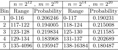
Theχ2goodness of fit test with 5 bins is used for evaluation. The probabilities used to derive the expected values are given in Table 6, and twop-values are produced for different versions.
Table 6.Ranges and probabilities of Collision Test for 16 and 20 bits
n= 212, m= 216 n= 214 , m= 220 Bin Range Probability Range Probability
1 0-116 0.206246 0-117 0.190231 2 117-122 0.194005 118-124 0.215008 3 123-128 0.219834 125-130 0.211585 4 129-134 0.183968 131-137 0.202689 5 135-4096 0.195947 138-16384 0.180487
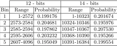
3.4 Coverage Test
Hash functions are one-way functions and required to behave like a random mapping, which implies that the expected coverage is about 63% of the size of the input set. The coverage test examines the size of the output set (coverage) formed from a subset of the domain.
The core of the test is as follows:
– A random message is taken and a set of size 212is formed by assigning all possible values to its first 12-bits.
– The output set of the compression function for this set is obtained.
– The coverage is computed, and the corresponding bin value is incremented by one. – These steps are repeated for 220different inputs.
– The same process is repeated for an input set of size 214.
Table 7.Ranges and probabilities of Coverage Test for 12 and 14 bits
12 - bits 14 - bits Bin Range Probability Range Probability
1 1-2572 0.199176 1-10323 0.201674 2 2573-2584 0.204681 10324-10346 0.195976 3 2585-2594 0.197862 10347-10367 0.207530 4 2595-2606 0.203232 10368-10390 0.195266 5 2607-4096 0.195049 10391-16384 0.199554
Similar to the statistical randomness tests, if p-value < 0,0001, we consider the data as non-random for the tests mentioned in this section. If p-value <0,001, we apply the test once more to check whether such a case is coincidental or not. If p-value < 0,001 is obtained again we consider the data as non-random.
4 Application
In this section, we apply statistical analysis to the SHA-3 second round candidate algorithms. For this purpose, first we define reduced versions of the candidates. Then, we apply statistical randomness tests and cryptographic randomness tests to observe the number of rounds that the algorithms achieve randomness.
When defining reduced versions of the algorithms, we only reduce the number of compression function rounds and ignore the finalization functions, if exist. Reduced rounds of finalization functions can also be taken into account, but this process together with the reduced rounds of compression functions increases the complexity of the tests by introducing plenty of versions for only one algorithm.
On the other hand, BMW and SHAvite-3 have two tunable parameters for the compression function that can be changed when reducing the algorithms. Therefore, to have a level testing field, we fix the first parameter and make the second one variable when defining the reduced versions of these algorithms. Also for SIMD, as the feed forward operation has a significant importance in the security of the algorithm, we do not exclude this operation in the reduced versions. Hence, 1 round of SIMD refers to 1 round of its compression function besides the feed forward operation.
For the sake of simplicity and ease of computations, we apply statistical analysis only to the 256-bit versions of the algorithms. In the case of cryptographic randomness testing, we apply the package directly to the compression functions of the candidate algorithms. Therefore, initialization and padding are excluded. In the case of statistical randomness testing, all the algorithms are tested for 256-bit output values, since the internal state size of the algorithms vary from 256 bits to 1600 bits and one needs to find the exact bin values of all the statistical randomness tests for each state size, which is not feasible.
4.1 Statistical Randomness Test Results
When applying statistical randomness tests to the candidates, we reduce the algorithms by excluding finalization, setting IV and salt values to 0. Moreover, we discard the padding operation and the output is generated from a single message block which is iterated only once.
Table 8.Statistical randomness test results for the 256-bit versions of the algorithms
Algorithm # Rounds # Rounds Random Data Sets
Blake [10] 10 3 Av1
BMW [11] 2/14 2/1 All
CubeHash [12] 16 6 LW
ECHO [13] 8 4 Av1
Fugue [14] 2 >2 All
Grøstl [15] 10 3 LW, HW, Av1, Rot
Hamsi [16] 3 1 All
JH [17] 35.5 8 LW, HW, Av1, Av8 Keccak [18] 24 3 LW, HW, Av1, Av8
Luffa [19] 8 3 LW, HW
Shabal [20] 3 1 All
Shavite3 [21] 3/12 3/1 All
SIMD [22] 4 1 All
Skein [23] 72 8 All
compression functions. However, we observe that two rounds ofG1 finalization or a single round of G2 finalization is enough for it to have random looking outputs.
4.2 Cryptographic Randomness Test Results
Different from statistical testing of the outputs of the algorithms, cryptographic randomness tests are applied directly to the compression functions of the candidate algorithms. As mentioned before in Section 3, the core operations of each test are advised to be repeated 220 times. However, especially in Coverage Test and Collision Test, 212 calls (or 214 calls depending on the chosen parameter) to the compression functions of the algorithms is required. This poses some limitations towards the number of times the cores of the tests can be repeated, since the performances of the reference codes provided in the submissions of the candidate algorithms vary significantly. Hence, we repeat the core operations of the tests as given in Table 9 to have reasonable running times for all algorithms.
Table 9.Number of times the core of the tests repeated with corresponding testing parameters
Test (Parameter) # Repetitions SAC Test (-) 220 Linear Span Test (-) 216 Collision Test (16) 216 Collision Test (20) 212 Coverage Test (12) 216 Coverage Test (14) 212
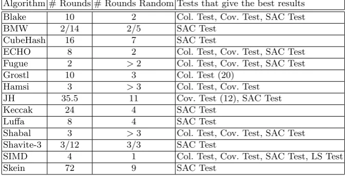
Table 10. Cryptographic randomness test results for the compression functions of the 256-bit versions of the algorithms
Algorithm # Rounds # Rounds Random Tests that give the best results Blake 10 2 Col. Test, Cov. Test, SAC Test
BMW 2/14 2/5 SAC Test
CubeHash 16 7 SAC Test
ECHO 8 2 Col. Test, Cov. Test, SAC Test Fugue 2 >2 Col. Test, Cov. Test, SAC Test Grostl 10 3 Col. Test (20)
Hamsi 3 >3 Col. Test, Cov. Test JH 35.5 11 Cov. Test (12), SAC Test
Keccak 24 4 SAC Test
Luffa 8 4 SAC Test
Shabal 3 >3 Col. Test, Cov. Test, SAC Test Shavite-3 3/12 3/3 SAC Test
SIMD 4 1 Col. Test, Cov. Test, SAC Test, LS Test
Skein 72 9 SAC Test
5 Conclusion and Future Work
In this work, we applied statistical randomness tests and cryptographic randomness tests on reduced round variants of the compression functions of the SHA-3 competition second round algorithms. We observed up to how many rounds a compression function behaves random. Al-though the results do not imply cryptographic weaknesses about the hash functions directly, it may provide a starting point for the cryptanalysis. The main outcome of this analysis is the knowledge of how conservative the algorithms are.
The results in Table 9 and Table 10 show how conservative the compression functions are. Ac-cording to these results Keccak, SIMD and Skein are the most conservative designs. On the other hand, the results obtained from Fugue, Shabal and Hamsi indicate relatively weak compression functions used for their designs. However they make up for this with use of cryptographically strong finalization functions.
As a future work, the analysis can be extended to other hash sizes. Moreover, finalization functions can be considered and more reduced versions can be constructed. Also new data sets can be defined for the statistical randomness testing.
References
1. National Institute of Standards and Technology. Announcing Request for Candidate Algorithm Nominations for a New Cryptographic Hash Algorithm (SHA-3) Family. Federal Register, 27(212):62212–62220, 2007. Available at: http://csrc.nist.gov/groups/ST/hash/documents/FR Notice Nov07.pdf.
2. Juan Soto and Jr. Randomness testing of the aes candidate algorithms.
3. Andrew Rukhin, Juan Soto, James Nechvatal, Elaine Barker, Stefan Leigh, Mark Levenson, David Banks, Alan Heckert, James Dray, San Vo, Andrew Rukhin, Juan Soto, Miles Smid, Stefan Leigh, Mark Vangel, Alan Heckert, James Dray, and Lawrence E Bassham Iii. A statistical test suite for random and pseudorandom number generators for cryptographic applications, 2001.
4. F. Sulak, A. Do˘ganaksoy, B. Ege, and O. Ko¸cak. Evaluation of randomness test results for short sequences. In Claude Carlet and Alexander Pott, editors,Sequences and Their Applications – SETA 2010, volume 6338 of Lecture Notes in Computer Science, pages 309–319. Springer Berlin / Heidelberg, 2010. 10.1007/978-3-642-15874-2 27.
5. Ali Do˘ganaksoy, Barı¸s Ege, Onur Ko¸cak, and Fatih Sulak. Cryptographic randomness testing of block ciphers and hash functions. Cryptology ePrint Archive, Report 2010/564, 2010. http://eprint.iacr.org/.
7. W. Caelli, E. Dawson, L. Nielsen, and H. Gustafson. CRYPT–X statistical package manual, measuring the strength of stream and block ciphers, 1992.
8. G. Marsaglia. The Marsaglia random number CDROM including the DIEHARD battery of tests of random-ness. 1996.
9. P. L’Ecuyer and R. Simard. Testu01: A c library for empirical testing of random number generators. ACM Trans. Math. Softw., 33(4):22, 2007.
10. Jean-Philippe Aumasson, Luca Henzen, Willi Meier, and Raphael C.-W. Phan. Sha-3 proposal blake. Sub-mission to NIST, 2008.
11. Danilo Gligoroski, Vlastimil Klima, Svein Johan Knapskog, Mohamed El-Hadedy, Jorn Amundsen, and Stig Frode Mjolsnes. Cryptographic hash function blue midnight wish. Submission to NIST (Round 2), 2009.
12. Daniel J. Bernstein. Cubehash specification (2.b.1). Submission to NIST (Round 2), 2009.
13. Ryad Benadjila, Olivier Billet, Henri Gilbert, Gilles Macario-Rat, Thomas Peyrin, Matt Robshaw, and Yan-nick Seurin. Sha-3 proposal: Echo. Submission to NIST (updated), 2009.
14. Shai Halevi, William E. Hall, and Charanjit S. Jutla. The hash function fugue. Submission to NIST (updated), 2009.
15. Praveen Gauravaram, Lars R. Knudsen, Krystian Matusiewicz, Florian Mendel, Christian Rechberger, Martin Schl¨affer, and Søren S. Thomsen. Grøstl – a sha-3 candidate. Submission to NIST, 2008.
16. ¨Ozg¨ul K¨u¸c¨uk. The hash function hamsi. Submission to NIST (updated), 2009. 17. Hongjun Wu. The hash function jh. Submission to NIST (updated), 2009.
18. G. Bertoni, J. Daemen, M. Peeters, and G. Van Assche. Keccak specifications. Submission to NIST (Round 2), 2009.
19. Christophe De Canniere, Hisayoshi Sato, and Dai Watanabe. Hash function luffa: Specification. Submission to NIST (Round 2), 2009.
20. Emmanuel Bresson, Anne Canteaut, Benot Chevallier-Mames, Christophe Clavier, Thomas Fuhr, Aline Gouget, Thomas Icart, Franois Misarsky, Mara Naya-Plasencia, Pascal Paillier, Thomas Pornin, Jean-Ren Reinhard, Cline Thuillet, and Marion Videau. Shabal, a submission to nists cryptographic hash algorithm competition. Submission to NIST, 2008.
21. Eli Biham and Orr Dunkelman. The shavite-3 hash function. Submission to NIST (Round 2), 2009. 22. Gatan Leurent, Charles Bouillaguet, and Pierre-Alain Fouque. Simd is a message digest. Submission to NIST
(Round 2), 2009.