Control of Pollution in River Streams

(1)

Control of Pollution in River Streams

Ogwola Peter,

Mathematical sciences Dept. Nasarawa State University, Keffi, Nasarawa

State , Nigeria. Peterogwola@yahoo.com 08032266281

Abstract

.

In industrial societies, rivers are used as dumps for sewage except that the sewage is treated at sewage stations prior to discharge into the stream. Untreated sewages discharged into the river contain high concentrations Biochemical Oxygen Demand (BOD) that has adverse effect on both human and aquatic organisms. The need of real-time monitoring and effective treatment of wastewater is urgent, and Dissolved Oxygen (DO) content in water quality monitoring is an important indicator. In this paper a methodology is presented to determine allowable concentrations of BOD in a wastewater discharge. A discrete dynamic model of first order difference equation is described for the dynamics of BOD and DO in a two reach river system. Kalman filtering technique is applied to the first order discrete dynamic model to estimate the concentrations of BOD in the effluent being discharged into the stream. This methodology was applied to Warri River in Delta state of Nigeria. It was observed that the maximum allowable

concentration of BOD in the effluent discharged to the stream is 0.01 mg/l.

Key

wards

:

River, DO, BOD, Pollution,

Sewage, Kalman filter, Control.

1.0 Introduction

In recent years there has been much interest in

regulating the levels of pollution in rivers. A good

measure of the quality of a stream is given by the

in-stream biochemical oxygen demand (B.O.D) and

the dissolved oxygen (D.O) in the stream.

If the D.O falls below certain level or the B.O.D

rises above certain level, fish die. In industrial

societies, rivers are used as dumps for sewage

except that the sewage is treated at sewage stations

prior to discharge into the stream (fig.1). Sewage

works in general operate a fixed level of treatment

which could be determined by the level of B.O.D in

the sewage which can be safely absorbed in the

stream. However, the ecological balance of the

river is often disturbed by unknown perturbations

and it becomes necessary to vary the B.O.D content

of the sewage (by increasing or decreasing the

(2)

back to the desired value. It is the problem of

on-line regulation of sewage discharge B.O.D from

multiple sewage works on polluted river that we

treat in this paper.

The river pollution control problem is essentially

how to control the BOD in the effluent discharge in

order to maintain desired levels of DO and BOD in

the river despite the stochastic effects (Singh and

Titli,1978)

Fig.1:Treated domestic wastewater being discharged into a stream (Penn M.Retal, 1999)

2.0 Definitions of Terms and Concepts

(i)Sewage-they are used water and waste

substances that are produced by human bodies and

carried away from houses and factories through

special pipes.

(ii)Effluent –is a treated wastewater, flowing from

treatment plant.

(iii)Biochemical oxygen demand (BOD)-a

parameter used to measure the rate of absorption of

oxygen by decomposing organic matter. The unit is

milligram per litre(mg/l)

(iv)Dissolve Oxygen (DO)-this is the amount of

oxygen dissolved (and hence available to sustain

marine life) in a body of water such as lake, river,

or stream. The unit is in milligram/ litre (mg/l).

(v)A reach of river-is defined as a stretch of a river

(3)

major effluent discharged from a sewage facility (fig. 2).

sewage

treatment discharged effluent

station

.

A reach of rive

Fig.2: A reach of river

(vi)A two reach river system-is a stretch of a river of some convenient length divided into two sections such that

each section receives one major effluent discharged from sewage facility (fig.3).

Sewage treatment Sewage treatment

Station 1 Station 2

discharged effluent. discharged effluent

1st_{reach of river} ₂nd_{reach of river}

Fig.3:A two reach river system

Previously, a number of river-water quality models have been developed for supporting waste loading

allocation, pollution control, and land-use planning in river basins (Guo etal, 2003).

The first water quality model was developed by Streeter and Phelps (1925). The basic principles behind this

model include (i) DO is supplied by reaeration and photosynthesis and demanded by respiration and BOD, and,

and (ii) BOD is due to emission from point and nonpoint sources and could be reduced by oxidation,

(4)

Beck and Young, 1976; Bowles and Grenney, 1978; DiCola et al, 1976; Eykhoff, 1974; Gnauk et al, 1976;

Koivo and Philips, 1972; Renaldi et al,1979; Moore and Jones, 1978).

3.0 The Kalman Filter

Kalman filter is defined as a set of mathematical equations that provides an efficient computational (recursive)

means to estimate the state of a process, in a way that minimizes the mean of the square error (Greg and Gary,

2006)

In order to use Kalman filter to estimate the internal state of a process, one must model the process in

accordance with the framework of the Kalman filter. This means specifying the following matrices:



, the

state-transition model, H, the observation model, Q, the covariance of the process noise, R, the covariance of the

observation noise; for each time step, k.

The Kalman filter model assumes the true state at time k is evolved from the state at (k-1) as stated below.

Xk =



Xk-1 +



k-1 (1)

Where



is the state transition model which is applied to the previous state Xk-1;



k is the process noise which is assumed to be drawn from a zero mean multivariate normal distribution

with covariance Qk,



k ~ N(0,Qk)

At time k an observation (or measurement) Yk of the true state Xk is made according to

Yk = HXk+



k (2)

Where H is the observation model which maps the true state space into the observed space and



k is the

observation noise which is assumed to be zero mean Gaussian white noise with covariance Rk ,



k~ N(0,Rk)

The initial state, and the noise vectors at each step



X

_o

,



₁

,...,



_k

,



,...



_k



are all assumed to be mutually

(5)

The Kalman filter is a recursive estimator. This means that only the estimated state from the previous time step

and the current measurement are needed to compute the estimate for the current state. No history of observations

and /or estimates is required. In what follows, the notation

1 | 



k k

X

which is the 1 step prediction represents the

estimates of

X

_k at time k given observations up to and including at time k-1.

| 1



k k

X

=



1 | 1 

 

k k

X

(3)

The covariance matrix for the one step prediction error is given by

p

Q

T k k k

k| 1





1| 1





₍₄₎

1 | 



k k

X

and Pk|k-1 are the Predicted(a priori) state estimate and Predicted(a priori) estimate of covariance

respectively and represent the initial values for the Kalman filter.

The state of the filter is represented by two variables

k k

X

_|



, the updated ( a posterior) state estimate at time k given observations up to and including at time k and

given by

X

k|k



= _| _₁



k k

X

+Kk(Yk−H _| ₁ 

k k

X

) (5)

Pk|k,, the updated( a posterior )error covariance matrix ( variance of the estimation error) given by

Pk|k = (I –KkH)Pk|k-1 (6)

Where Kk is the Kalman (Filter) gain and given by

Kk = Pk|k-1HT(H Pk|k-1HT +R)-1 (7)

In Fig. 4, Kalman filter is summarized as Kalman Filter Loop(Robert and Patrick, 1992). Once the loop is

(6)

Enter prior estimate



X

k|k-1and its covariance Pk|k-1

Fig.4:The Kalman Filter Loop (Robert and Patrick, 1992)

4.0 Discrete-time Linear- Quadratic-Gaussian (LQG) Problem

Consider the dynamic system,

Xk+1 =



X

_k



BU

_k+



_k

(8)

Yk = HXk+



_k

Where

X

_k is an n-vector ,

U

k is an m-vector (

m



n

)

,



,

B

are n x n resp. n x m matrices whose elements

are non-random functions of time. Given the observed values of Y0,…..,Yk, we are to find a sequence

U1,U2,…….,Uk of control vectors that minimizes the performance index

J = _k _kT _k N

k T

k

QX

U

RU

X









1

0 (9)

Compute kalman gain

Kk = PK|K-1 HT (HPK|K-1 HT + R)-1

Update estimate with measurement yk



X

k|k=



X

k|k-1+ KK(yk– H



X

k|k-1

)

Compute covariance matrix for updated

estimate

Pk|k= (1-EKH)PK|K-1

Project ahead



X

K+1|K = ф



X

k|k

(7)

Where Q , R are symmetric and positive definite matrices whose elements are non-random functions of time, N

is the number of iterations.

The discrete-time controller is

Uk = − GXk (10)

5.0 Theorem

:

Separation Principle

In control theory, a separation theorem, more formally known as theorem of separation of estimation and

control, states that under some assumptions the problem of designing an optimal feedback controller for a

stochastic system can be solved by designing an optimal observer for the state of the system, which feeds into an

optimal deterministic controller for the system (fig.5). Thus the problem can be broken into two separate parts,

which facilitates the design (Wikipedia)

This result is the celebrated separation theorem of linear stochastic control and was proved independently by

Joseph and Tou (1961) and Gunkel and Franklin (1963).

Fig. 5

Fig.5: Observer-based controller(Grewal and Andrews, 2010)

6.0 The Warri River

The Warri river in Delta State of Nigeria is an example of inland water receiving sewage from several

industries, factories and markets. These wastes often contain significant spectrum of organic and inorganic

substances capable of producing adverse effects on the physical, chemical and biotic components of the

Dynamics _sensors

Deterministic optimal

controller Kalman filter

u

x

z

Stochastic control system

(8)

environment either directly or indirectly on human health (Aghoghovwia, 2008). The rapid increase in human

population, inadequate infrastructural facilities, lack of good/proper facilities for waste disposal as well as

problem of refuse collection and disposal, have contributed to the environmental decay (Odiete, 1990). Warri

River flows through the adjourning mangrove swamp forest area of the southern part of Nigeria, where the

drainage and catchment areas are probably very rich in decaying organic matter and humus. Warri River

stretches within latitude 50₂₁’_{to 6}0₀₀’_{N and longitude 5}0₂₄’_{to 6}0₂’_{E. Its source is around Utagba Uno, covering}

a surface area of above 255 km2_{with a length of about 150 km. From its source, the river flows South-westerly}

direction passing between Oviorie and Ovu-inland and southwards at Odiete through Agbarho to Otokutu and

Ugbolokposo (Egborge, 2001) It turns southwards to Effurun and forms a ‘W’ between Effurun and Warri.

Important land marks in this River stretch are Enerhen, Igbudu, Ovwian and Aladja(steel town),Warri ports,

main Warri market, NNPC Refinery, Globe star, etc.

Warri River was chosen as a case study for this research for the following reasons:

i) There are several industries, factories and markets within Warri as such Warri River is subject to large

quantity of sewages flowing into it which causes a large quantity of pollution in the River.

ii) Many Researchers are interested in studying the amount of pollution in Warri River because of the above

reason.

iii) This pollution produces adverse effects on the physical, chemical and biotic components of the environment

either directly or indirectly on human health and so it needed to be controlled.

Many Researchers worked on Warri River to determine the quantity of the pollution, such as: Arimoro et al;

Aghoghoviwia,2011; Aghoghovwia,2008; Olomukoro et al,2009; Edegbene et al,2012.

(9)

Fig.6: Map showing Warri River (Aghoghovwia, 2008)

Reach 1 of the river covers the 500 metres length of the river along Naval base and Reach 2 which started from

the end of Reach 1 covers the 500 metre length of the river along Main Warri Market.

7.0 Formulation of the two reach River model.

Beck (1978) presented a single reach model given by:

































  

i i i i i i

E i i i i i s i i i

i E i i i

E i i i i i i i

v

z

k

q

v

Q

q

v

Q

q

k

q

v

Q

z

v

Q

z

v

Q

z

k

z





1 1

1 2

1 1 1

)

(

(11)

Where,

zi , zi-1 are the concentrations of B.O.D. in reaches i and i-1 in mg/litre

qi , qi-1 are the concentrations of D.O. in reaches i and i-1 in mg/litre

vi is the volume of water in reach i in million gallons

QE is the flow rate of the effluent in reach i in million gallons/day

kli is the oxygen consumption coefficient(day)-1 in reach i

k2i is the oxygen recovery coefficient(day)-1 in reach i

Qi , Qi-1 are the stream flow rates in reaches i and i-1 in million gallons/day

qis is the D.O. saturation level for the ith reach (mg/litre)

i i

v



is the removal of D.O. due to bottom sludge requirements (mg/litre(day)-1₎

i

(10)

E i

Q



Fig.7:Flow diagram for Becks model.

A two reach river model is formulated as an extension of a single reach model. The stretch of the river is

divided into two reaches (reach 1 and reach 2). Model equations for reach 1 and reach 2 were formulated

independently and then merged together to form four order state space equation. Reach 1 is designated as i1 and

Reach 2 is designated as i2.

7.1 Model Equation for Reach 1

dt

dz

i₁

= −𝑘 1 1

1i

z

i + 11 1

1 1

 

i i i

z

v

Q

−

1 1

1

)

(

i i

E i

z

v

Q



+

1 1 1

i E i

v

Q



(12)

1 1 1 1 1 1

1 1 1 1 1

1 1 1 1 1 1 1

1 2

2

)

(

i i i i i i

E i i

i i i i s i i i

v

z

k

q

v

Q

q

v

Q

q

k

q

k

dt

dq















 _

Where,

,

1

i

z

1 1

i

z

are the concentrations of B.O.D. in reaches

i

₁ and

i

₁_₁ in mg/litre

,

1

i

q

1 1

i

q

are the concentrations of D.O. in reaches

i

₁ and

i

₁_₁ in mg/litre

Reach i-1 Reach i

zi-1

qi-1

Qi-1

zi

qi

Qi

QE

i



K1

i

K2iqis _K

(11)

1

i

v

is the volume of water in reach

i

₁ in million gallons

1

E

Q

is the flow rate of the effluent in reach

i

₁ in million gallons/day

1

1i

k

is the oxygen consumption coefficient(day)-1_{in reach}

1

i

1

2i

k

is the oxygen recovery coefficient (day)-1_{in reach}

1

i

,

1

i

Q

1 1

i

Q

are the stream flow rates in reaches

i

₁ and

i

₁_₁ in million gallons/day

s i

q

1 is the D.O. saturation level for the

th

i

₁ reach (mg/litre)

1 1

i i





1

i



is the concentration of B.O.D. in the effluent in mg/litre

Fig.7: Flow diagram for reach 1

1 1

i

z

1 1

i

q

1 1

i

Q

Reach

i

₁

Reach

i

₁_₁

1 1 E

i

Q



1

1i

k

1

i



1

2i

k

s i i

q

k

1 1

2

1

E

Q

1

i

z

1

i

q

1

i

(12)

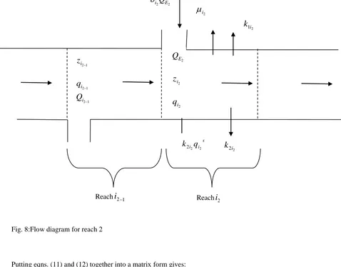
7.2 Model Equation for Reach 2

dt

dz

_i 2 = −𝑘 2 2

1i

z

i + 21 2 1 2   i i i

z

v

Q

− 2 2 2 2

)

(

i i E i

z

v

Q



+ 2 2 2 i E i

v

Q



(13) 2 2 2 2 2 2 2 2 1 2 2 1 2 2 2 2 2 2 1 2 2

)

(

i i i i i i E i i i i i i s i i i

v

z

k

q

v

Q

q

v

Q

q

k

q

k

dt

dq















 _ Where,

,

2 i

z

1 2 i

z

are the concentrations of B.O.D. in reaches

i

₂ and

i

₂_₁ in mg/litre

,

2 i

q

1 2 i

q

are the concentrations of D.O. in reaches

i

₂ and

i

₂_₁ in mg/litre

2

i

v

is the volume of water in reach

i

₂ in million gallons

2

E

Q

s the flow rate of the effluent in reach

i

₂ in million gallons/day

2

1i

k

is the oxygen consumption coefficient(day)-1_{in reach}

2

i

2

2i

k

is the oxygen recovery coefficient(day)-1_{in reach}

2

i

,

2 i

Q

1 2 i

Q

are the stream flow rates in reaches

i

₂ and

i

₂_₁ in million gallons/day

s i

q

2 is the D.O. saturation level for the

th

i

₂ reach (mg/litre)

2 2 i i





2

i



is the concentration of B.O.D. in the effluent in mg/litre

(13)

Fig. 8:Flow diagram for reach 2

Putting eqns. (11) and (12) together into a matrix form gives:













dt

dq

dt

dz

dt

dq

dt

dz

i i i i 2 2 1 1 =









































2 2 1 1 2 2 2 2 2 2 2 2 2 1 1 1 1 1 1 1 1 1

(

0

0 )

(

0

0 )

(

0

0 )

(

2 1 1 2 1 1 i i i i i E i i i i E i i i E i i i i E i i

q

z

q

z

v

Q

k

v

Q

k

v

Q

k

v

Q

k

+ 1 2 i

z

1 2 i

q

1 2 i

Q

Reach

i

₂

Reach

i

₂_₁

(14)

























2 1 2 2 1 1

0

i i i E i E

v

Q

v

Q



+





















































        2 2 2 2 1 1 1 1 1 2 1 2 1 1 1 1 2 1 2 2 1 2 1 1 1 1 1 1 2 2

0

i i s i i i i s i i i i i i i i i i i i i i

v

q

k

v

q

k

q

z

q

z

v

Q

v

Q

v

Q

v

Q



(14)

Equation (14) is represented by first order deference equation of the form:

Xk+1 =



Xk + BUk+ C (15)

Where:



=





























2 2 2 2 2 2 2 2 2 2 1 1 1 1 1 1 1 1

)

(

0

0 )

(

0

0 )

(

0

0 )

(

2 1 1 2 1 1 i E i i i i E i i i E i i i i E i i

v

Q

k

v

Q

k

v

Q

k

v

Q

k

(16)

Xk =













2 2 1 1 i i i i

q

z

q

z

(17) B =













0

2 2 1 1 i E i E

v

Q

v

Q

(18)

(15)

C =





















































        2 2 2 2 1 1 1 1 1 2 1 2 1 1 1 1 2 1 2 2 1 2 1 1 1 1 1 1 2 2

0

i i s i i i i s i i i i i i i i i i i i i i

v

q

k

v

q

k

q

z

q

z

v

Q

v

Q

v

Q

v

Q



(20)



, B, Xk, Uk, is the transition model, the control input model, the process state vector and the control vector

respectively. C is a constant matrix.

8.0 Optimal Control Problem.

The optimal control problem is then stated as follows:

Minimize J = _k _kT _k

N k

T

k

QX

U

RU

X









1

0 (21)

Subject to: Xk+1 =



X

_k



BU

_k+



_k

Yk = HXk+



_k

Where:



= ( 4× 4) constant matrix obtained from the transition model

B = ( 4× 2) control input matrix which is applied to the control vector Uk .

Yk = ( 2× 1) output vector (vector measurement at time tk ), Yk=













2 1

y

, y1 is the measured D.O in reach 1 and y2

is the measured D.O in reach 2 of the stream.

H = ( 2× 4) constant matrix giving the ideal connection between the measurement and the

(16)

Xk= (4× 1) process state vector at time tk , i.e.,Xk =X (tk) =













4 3 2 1

x

, x1 and x3 are the concentrations of

B.O.D.( mg/l) in reaches 1 and 2 of the stream and x2 , x4 are the concentrations of D.O in reaches 1 and 2 of

the stream.

Uk = ( 2× 1) control vector, Uk=













2 1

u

, where u1 and u2 are the concentrations of B.O.D in the effluent to

reaches 1 and reach 2 of the stream.



k = ( 2× 1) measurement error –assumed to be white noise sequence with known co-

Variance R and having zero cross correlation with



ksequence.



k= ( 4× 1) vector-assumed to be white noise sequence with known co-variance Q

Note that x2 and x4 are the estimates of the true value of D.O in Reach 1 and 2 of the stream, y1 and y2 are the

measured value of D.O in reach 1 and 2 of the stream.

9.0 D

.O Measurements

The DO measurements Yk =













2 1

y

at tk , where y1and y2 are the concentrations of DO in reach 1 and reach 2 of

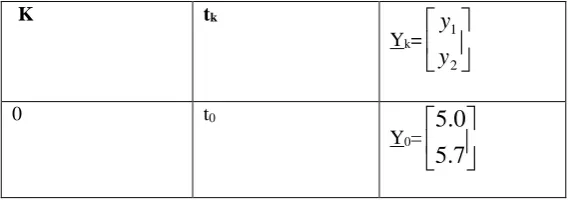
the river as given in Table 2.

Table 2:

D.O Measurements, Y

k

at time t

K

(Aghoghovwia, 2011).

K tk

Yk=













2 1

y

0 t0

Y0=













7 .

5

(17)

1 t1

Y1=













3 .

5

0 .

6

2 t2

Y2=













3 .

6

5 .

5

3 t3

Y3=













6 .

6

4 .

5

4 t4

Y4=













3 .

7

7 .

6

5 t5

Y5=













0 .

8

0 .

7

6 t6

Y6=













1 .

6

5 .

6

7 t7

Y7=













5 .

7

2 .

6 T

able1:

Parameter Values for Warri river Model at 29

o

_{C( Ogwola,2017)}

Symbol Value Sources

L1

L2

W1

W2

D1

D2

1

i

Q

2

i

Q

1

i

v

2

i

v

500 metres

150 metres

7.5 metres

0.643m3_{/s(14672937.5 gallons/day)}

562500m3_{(148597242.04 gallons)}

Ogwola,2017

,,

(18)

ASSUMPTIONS[with respect to Guo et al (2003)] 1 E

Q

2 E

Q

1 1i

k

2 1i

k

1 2i

k

2 2i

k

0.659m3_{/s(15046510.9 gallons/day)}

1 2 2 3 Assumption ,, ,, ,, ,, ,,

With respect to table 1, values of



and B were obtained from (15) and (17) respectively.



=















0 .

3

0 .

2

0

2 .

2

0

2 .

2

0 .

1

0

2 .

1

B =













0

1 .

0

1 .

0

The process variance Q and the measurement variance R were tuned to:

Q =













2

0

2

0

2

0

2

and R =













2

0

2

The control system tool box function [G,S] = LGR(



,B,Q,R) is used to compute the optimal gain matrix G.

G =

_













0058

.

0 0280

.

0 0000

.

0 0000

.

0 0000

.

0 0000

.

0 0067

.

0 0471

.

0

With respect to Kalman filter Tank filling the initial values X0|0 and P0|0 are:

X0|0 =













0

P0|0 =

(19)

H which is the constant matrix that gives ideal connection between the measurement and the state vector is

given by:

H =













1

0

1

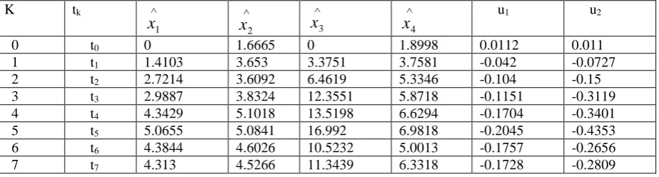
0 Table 3:

The Simulation Results for the System

K tk 

1

x

₂



3

x



4

x

u1 u2

0 t0 0 1.6665 0 1.8998 0.0112 0.011

1 t1 1.4103 3.653 3.3751 3.7581 -0.042 -0.0727

2 t2 2.7214 3.6092 6.4619 5.3346 -0.104 -0.15

3 t3 2.9887 3.8324 12.3551 5.8718 -0.1151 -0.3119

4 t4 4.3429 5.1018 13.5198 6.6294 -0.1704 -0.3401

5 t5 5.0655 5.0841 16.992 6.9818 -0.2045 -0.4353

6 t6 4.3844 4.6026 10.5232 5.0013 -0.1757 -0.2656

7 t7 4.313 4.5266 11.3439 6.3318 -0.1728 -0.2809

Where



1

x

is the optimal estimate of BOD in Reach 1 of the river in milligram per litre(mg/L)



2

x

_{is the optimal estimate of DO in Reach 1 of the river in mg/litre}



3

x

is the optimal estimate of BOD in Reach 2 of the river in mg/litre



4

x

_{is the optimal estimate of DO in Reach 2 of the river in mg/litre}

u1 is the concentration of BOD in the effluent to Reach 1in mg/litre

u2 is the concentration of BOD in the effluent to Reach 2 in mg/litre

(20)

The results of this research showed that the average estimated values of BOD (x1) in Reach 1(column 3 of

Table 3) is 3.1533 mg/l and the average estimated values of BOD (x3) in Reach 2(column 5 of Table 3) is

9.3214 mg/l. This shows that the BOD varies with respect to locations in this river.

According to Wikipedia, ‘unpolluted rivers have BOD below 1 mg/l’. The average concentration of BOD in

Reach 1 and Reach 2 is 3.1533 mg/l and 9.3214 mg/l respectively, therefore Warri river is polluted and not

suitable for drinking.

With respect to the Water Quality Assessment and Pollution Control ,Reach 2 is not a suitable environment for

fish growth since the BOD value of 9.3214 mg/l is greater than 4mg/l. The BOD values in Reach 2 of the stream

exceeded stipulated permissible limit for drinking and for protection of health in fish which is also in line with

Aghoghovwia (2011).

Effluent is a treated wastewater flowing from treatment plant into a river. The concentration of BOD in the

effluent determines the level of treatment of the sewage. If an effluent has BOD of less than 1 mg/l then it is

unpolluted and suitable for discharging into the stream.

With respect to the assumption that the flow rate of the effluent to the river is 15046510.9 gallons/day the results

of this research show that the maximum concentration of BOD in the effluent to Reach1(u1) is 0.0112

mg/l(seventh column of table 3) and the maximum concentration of BOD in the effluent to Reach2(u2) is 0.0110

mg/l(eighth column of table 3). These values are less than 1 mg/l of BOD and therefore the effluents are

unpolluted and safe for discharging into the stream.

Therefore, the sewage must be treated to a level such that the concentration of effluent from sewage must not

exceed 0.011 mg/l of BOD.

11.0 Conclusion

The fact that emerged from this study is that the level of BOD in Warri river exceeded the stipulated permissible

limit for drinking water and to protect health of fish, sewages need to be treated to the desired level before

discharging into the river to avoid stream pollution.

(21)

Aghoghovwia, O.A (2011). Physico-chemical Characteristics of Warri River in the Niger Delta Region of Nigeria. Journal of Environmental Issues and Agriculture

in Developing Countries, Vol. 3, No. 2.

Aghoghovwia, O.A (2008). Assessment of industrial and Domestic Effects on

Fish Species Diversity of Warri River, Delta State, Nigeria. Ph.D Thesis submitted to the University of Ibadan, Ibadan, Nigeria. Pp. 1-111.

Arimoro, F.O; Iwegbue,C.M.A and Osiobe,O (2008). Effect of Industrial Waste Water on the Physical and Chemical characteristics of a Tropical Coastal River.. Research Journal of

Environmental Sciences, 2: 209-220.

Beck,M.B (1978).A Comparative Case Study of Dynamic Models DO-BOD-Algae Interaction in Freshwater River. International Institute for Applied Systems Analysis,RR-78-19.

Edegbene, A.O; Arimoro, E.O; Nwaka, K.H; Omovoh, G.O; Ogidiaka, E and Abolagba, O.J(2012) The Physical and Chemical Characteristics of Atakpo River, Niger Delta, Nigeria.

Journal of Aquatic Sciences. 27 (2): 159-172.

Greg,W and Gary,B (2006).An introduction to the Kalman Filter.TR 95-041 Department of Computer Scienc University of North Carolina at Chapel Hill,Chapel Hill,NC 27599-3175.

Gunkel, T. and Franklin, G (1963). “A general solution for linear sampled data control”. J. Basic Eng. Vol. 85, p. 197.

Joseph, P. and Tou, J. (1961). “On Linear control theory”. Trans. AIEE pt II, vol. 80, pp. 193-196.

Kalman, R.E (1960). A New Approach to Linear Filtering and Prediction Problems. Journal of Basic Engineering 85, 95-108.

Kalman Filter Tank Filling (M163) :

https://www.cs.cornell.edu/courses/cs4758/2012sp/material/mi63slides.pdf

Odiete,W.O (1990).Environmental Physiology of Animals and Pollution. Lagos: Diversified Resources Limited.

Ogwola,P.(2017).Application of the Kalman Filtering Technique for Controlling the

Problems of River Pollution(A Case Study of Warri River). Ph.D.Thesis, Nasarawa State university.

Olomukoro, J.O; Osunde, G.A and Azubuike, C.N(2009) Eichhornia Crassipes invasion and Physicochemical Characteristics of a Creek flowing through an urban area in Southern Nigeria. African Scientist Vol. 10, No. 1 .

Pregun, C and Juhász, C (2011). Water Resources Management and Water Quality Protection.

Robert, G. B and Patrick, Y. C. H (1992).Introduction to Random Signals and Applied Filtering. Hamilton Printing Company.

(22)

Pergamon Press Oxford.

Streeter, H.W. and Phelps,E.B(1925). A study on the pollution and natural purification of the Ohio River, US Public Health Service, Public Health Bulletin, No, 146, Washington, DC, USA.

Wikipedia:.https://en.wikipedia.org/wiki/Biochemical

Wikipedia: https://en.wikipedia.org/wiki/separation_principle

Water Quality Assessment and Pollution:

http://repository.fuoye.edu.ng/bitstream/123456789/750/1/water%20Quality%20Assessment%20and%20Polluti

on%20Control%.pdf