Scholarship@Western
Scholarship@Western
Electronic Thesis and Dissertation Repository
9-26-2018 10:00 AM
Statistical tools for assessment of spatial properties of mutations
Statistical tools for assessment of spatial properties of mutations
observed under the microarray platform
observed under the microarray platform
Bin Luo
The University of Western Ontario
Supervisor Dean, Charmaine
The University of Western Ontario Joint Supervisor Kulperger, Reg
The University of Western Ontario
Graduate Program in Statistics and Actuarial Sciences
A thesis submitted in partial fulfillment of the requirements for the degree in Doctor of Philosophy
© Bin Luo 2018
Follow this and additional works at: https://ir.lib.uwo.ca/etd
Part of the Biostatistics Commons
Recommended Citation Recommended Citation
Luo, Bin, "Statistical tools for assessment of spatial properties of mutations observed under the microarray platform" (2018). Electronic Thesis and Dissertation Repository. 5746.
https://ir.lib.uwo.ca/etd/5746
This Dissertation/Thesis is brought to you for free and open access by Scholarship@Western. It has been accepted for inclusion in Electronic Thesis and Dissertation Repository by an authorized administrator of
Mutations are alterations of the DNA nucleotide sequence of the genome. Analyses of
spatial properties of mutations are critical for understanding certain mutational mechanisms
relevant to genetic disease, diversity, and evolution. The studies in this thesis focus on two
types of mutations: point mutations, i.e., single nucleotide polymorphism (SNP) genotype
dif-ferences, and mutations in segments, i.e., copy number variations (CNVs). The microarray
platform, such as the Mouse Diversity Genotyping Array (MDGA), detects these mutations
genome-wide with lower cost compared to whole genome sequencing, and thus is considered
for suitability as a screening tool for large populations. Yet it provides observation of
muta-tions with high degree of missingness across the genome due to its design, which thus leads to
challenges for statistical analyses. Three topics are studied in this thesis: the development of
formal statistical tools for detecting the existence of point mutation clusters under the
microar-ray platform; the evaluation of the performance of test statistics developed while accounting
for various probe designs, in terms of the capabilities of detecting mutation clusters; the
de-velopment of formal statistical tools for testing the existence of spatial association between
point mutations and mutations in segments. Statistical models such as Poisson point processes
and Neyman-Scott processes are used for the distributions of the locations of point mutations
under null and alternative hypotheses. Monte Carlo frameworks are established for statistical
inference and the evaluation of power performance of the proposed test statistics. Tests with
desirable performance are identified and recommended as screening tools. These statistical
tools can be used for the study of other genomic events in the form of point events and events
in segments, as well as with other microarray platforms than the MDGA which is utilized
here. Simulated probe sets based on a window-based probe design mimicing the design of the
MDGA are used to study the effect of various factors in probe design on the performance of
test statistics. Insights are offered for determining key features in such design, such as probe
intensity, when designing a new microarray platform, in order to achieve desired power for the
purpose of mutation cluster detection.
pothesis testing; Missing data; Genomics; Mutation shower; Single nucleotide polymorphism;
Copy number variation; Microarray probe design sampling; Mouse Diversity Genotyping
Ar-ray
This work was completed under the supervision of Dr. Charmaine Dean and Dr. Reg
Kulperger, and with collaboration of Dr. Kathleen Hill. All papers resulting from this thesis
will be co-authored with Drs. Dean, Kulperger and Hill.
First and foremost, I would like to express my deepest gratitude and appreciation to my
supervisors, Dr. Charmaine Dean nad Dr. Reg Kulperger. I would like to thank them for
providing me the opportunity to become their student while I was searching for supervisors,
and giving me the freedom to choose a research area I am interested in. This thesis would
not have been in any way possible without their mentorship, guidance, support, kindness, and
patience. It is my greatest pleasure and honor to be their student. I would also like to give
my most sincere gratitude to our collaborator, Dr. Kathleen Hill. I would like to thank her for
her introduction to many interesting biological research questions, and her tremendous support
throughout my study.
I am thankful to my M.Sc. supervisor Dr. Ian McLeod, and my previous Ph.D. supervisor
Dr. Jiguo Cao, who led me to research in statistics. I would also like to thank all the graduate
chairs in our department during my M.Sc. and Ph.D. studies. Special thanks to Dr. John Braun
who encouraged me to join the program and provided me with valuable suggestions, and Dr.
Marcos Escobar-Anel who assisted with rules of School of Graduate and Postdoctoral Studies.
I would like to express special gratitude to the lab of Dr. Charmaine Dean and Dr. Doug
Woolford. I benefit greatly from the excellent academic environment built by all lab members.
I would also like to thank all the lab members from Dr. Kathleen Hill’s lab. The discussion and
communication with them provided valuable help to my research.
I am grateful to my course instructors from both the Department of Statistical and Actuarial
Sciences and the Department of Epidemiology and Biostatistics. Their courses helped me build
foundation in statistical knowledge and develop an interest in research.
I would like to express special appreciation to all the assistants of Dr. Charmaine Dean,
who did a fantastic job helping me arrange meeting schedules. My appreciation also goes to
the administrative staffin the Department of Statistical and Actuarial Sciences.
I highly appreciate the Engage Grant and Mitacs Accelerate programs for providing me the
opportunity to gain industrial experience during my study. I would like to thank the colleagues
ment. The research experience I gained from this collaboration became very helpful during my
Ph.D. research.
Many thanks are due to all the friends I have made here in London. Their company, help
and support have been invaluable to me to allow me to live a good and happy life. Special
thanks to Rosie and Bilbo whose accompany made my life more colorful.
Finally, my greatest gratitude and appreciation extend to my family: my parents, Jisheng
Luo and Chunying Xia, and my wife, Yue Cai. Without their unconditional love and support,
I would not have been able to achieve anything during my study. I wish that all of them could
see this completion of my degree.
Certificate of Examination i
Abstract i
Co-Authorship Statement iii
Dedication iv
Acknowlegements v
List of Figures xi
List of Appendices xvi
1 Overview 1
2 Spatial statistical tools for genome-wide mutation cluster detection under a mi-croarray probe sampling system 7
2.1 Introduction . . . 8
2.2 Methods . . . 13
2.3 Small sample properties of the test statistics . . . 19
2.3.1 Proposed underlying processes for the null hypothesis . . . 19
2.3.2 Proposed underlying processes for alternative hypotheses . . . 22
2.3.3 Simulation parameter settings and results . . . 26
2.4 Application . . . 34
2.4.2 Analyses for three biological samples of interest . . . 35
2.5 Discussion . . . 37
3 Effect of probe design in microarray type data on powers of test statistics for cluster detection 42 3.1 Introduction . . . 43
3.2 Statistical methods . . . 45
3.2.1 Probe sets designed from simulated libraries . . . 46
3.2.1.1 Library generation . . . 46
3.2.1.2 Window-based probe selection procedure . . . 48
3.2.2 Probe sets filtered from MDGA . . . 50
3.2.3 Methodology for power study . . . 50
3.3 Power study . . . 53
3.3.1 Parameter settings . . . 53
3.3.2 Power comparisons . . . 54
3.4 Discussion . . . 63
4 Nonparametric association test for spatial independence in the occurrence of single nucleotide polymorphism differences and copy number variations under a microarray probe sampling system 66 4.1 Introduction . . . 67
4.2 Statistical methods . . . 69
4.2.1 Data structure . . . 69
4.2.2 Proposed statistics . . . 70
4.3 Small sample properties of the test statistics . . . 71
4.3.1 Monte Carlo simulation approaches for inference . . . 72
4.3.1.1 Poisson null process . . . 73
4.3.1.3 Partial block bootstrap . . . 76
4.3.2 Statistical inference . . . 76
4.3.3 Alternative processes for power studies . . . 78
4.3.3.1 Step function nhPP . . . 78
4.3.3.2 Modified non-homogeneous parent Neyman-Scott process (NPNSP) 79 4.3.4 Parameter settings and simulation results . . . 80
4.3.4.1 Parameter settings for confidence band construction . . . 80
4.3.4.2 Parameter settings for power study . . . 81
4.3.4.3 Power study results, interpretation, and recommendation . . . 81
4.4 Application . . . 91
4.5 Discussion . . . 98
5 Summary and future work 102 Bibliography 105 A Supplementary information for Chapter 2 111 A.1 Validation of size of test statistics . . . 111
A.1.1 Scheme a . . . 111
A.1.2 Scheme b . . . 113
A.2 Additional power study figures . . . 115
B Supplementary information for Chapter 3 118 C Supplementary information for Chapter 4 121 C.1 Geometrical illustration of the partial block bootstrap . . . 121
C.2 Parameter setting in the alternative hypothesis for the step function nhPP model 124 C.3 Examination of autocovariance for location of SNP differences on microarray data . . . 125
D.1 Monte Carlo simulation for statistical inference and power estimation . . . 128
D.2 Block bootstrap for dependent data . . . 129
D.3 DNA data structure: discreteness . . . 130
D.4 Spatial point process . . . 131
D.5 Notes on numerical computation . . . 132
Curriculum Vitae 133
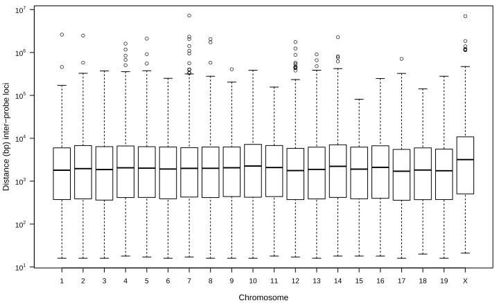
2.1 The inter-SNP locus distances (bp) for 493,290 SNP loci assayed by the probes
on the Mouse Diversity Genotyping Array (MDGA) are summarized for each
chromosome. . . 11
2.2 Power performance of statistics related to ¯R(d), ˜R(d), andC(d) under alternative
hypothesis (1) with parameterµo =375. . . 28
2.3 Power performance of statistics related to ¯R(d), ˜R(d), andC(d) under alternative
hypothesis (2) with parameterµo =375. . . 29
2.4 Power performance of statistics related to ¯R(d), ˜R(d), andC(d) under alternative
hypothesis (3) with parameterµo =375. . . 30
2.5 Power performance of test statistics ˜R(d) across a grid of d under alternative
hypothesis (1) with parameterµo =375. . . 33
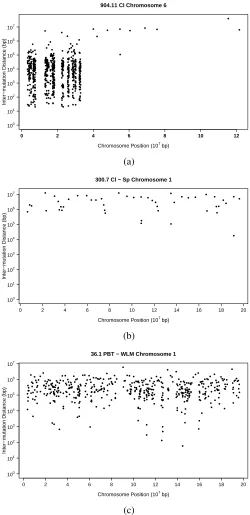
2.6 Rainfall plots portraying the SNP differences due to mixed genetic background,
putative new mutations arising during development of two normal tissues of the
same mouse and putative mutations arising between two cancerous tissues from
the same mouse. . . 36
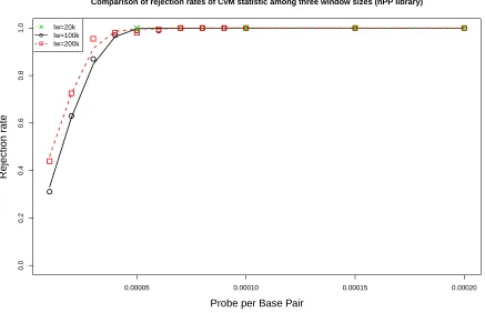
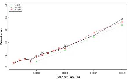
3.1 Comparison of rejection rates of CvMR˜ under various probe settings among
three window sizes. The mouse library is constructed from hPP samples. . . 56
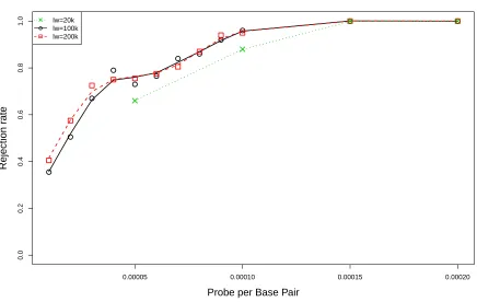
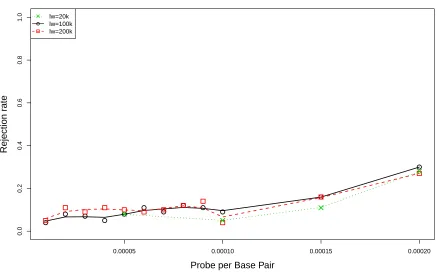
3.2 Comparison of rejection rates ofKSR˜ under various probe settings among three
window sizes. The mouse library is constructed from hPP samples. . . 57
3.3 Comparison of rejection rates of CvMR˜ under various probe settings among
three window sizes. The mouse library is constructed from NS samples. . . 58
window sizes. The mouse library is constructed from NS samples. . . 59
3.5 Comparison of rejection rates ofCvMR˜ under filtered probe sets based on
chro-mosome 19, hPP library (lw = 100k) and NS library (lw = 100k). The blue
and black dashed vertical lines indicate probe intensities required for high
per-formance with the hPP library and filtered probe sets on chromosome 19 from
MDGA respectively. . . 60
3.6 Comparison of rejection rates ofKSR˜ under filtered probe sets based on
chro-mosome 19, hPP library (lw= 100k) and NS library (lw =100k). . . 61
4.1 The first two steps of the overall block bootstrap are illustrated. Sample a point
g1 ∼ U(sf,sl) on the original chromosome. All SNP differences and probes
within the segment [g1,g1+BO−1] on the original chromosome are relocated
to the segment [sf,sf+BO−1] on the resampled chromosome, maintaining their
exact position relative tog1, but now fromsf on the resampled chromosome. A
subsequent pointg2 ∼ U(sf,sl) is taken on the original chromosome, the SNP
differences and probes within [g2,g2 + BO − 1] are relocated to the segment
[sf +BO,sf +2BO−1] on the resampled chromosome, again maintaining their
exact position relative tog2, but now fromsf+BOon the resampled chromosome. 75
4.2 Power performance ofJandCstatistics under the alternative hypothesis of the
step function nhPP using confidence bands constructed from the Poisson Null
Process. . . 83
4.3 Power performance ofJandCstatistics under the alternative hypothesis of the
step function nhPP using confidence bands constructed from the overall block
bootstrap. . . 84
4.4 Power performance ofJandCstatistics under the alternative hypothesis of the
step function nhPP using confidence bands constructed from the partial block
bootstrap. . . 85
modified NPNSP using confidence bands constructed from the Poisson Null
Process. . . 86
4.6 Power performance ofJandCstatistics under the alternative hypothesis of the
modified NPNSP using confidence bands constructed from the overall block
bootstrap. . . 87
4.7 Power performance ofJandCstatistics under the alternative hypothesis of the
modified NPNSP using confidence bands constructed from the partial block
bootstrap. . . 88
4.8 Rainfall plot displaying mutation landscapes. Black dots refer to SNP diff
er-ences. Red markers identify CNV locations. The green dashed vertical lines
show the centers of the CNVs. . . 92
4.9 Rainbow plot displaying mutation landscapes. Black dots refer to SNP diff
er-ences. Red markers identify CNV locations. The green dashed vertical lines
show the centers of the CNVs. . . 93
4.10 J statistic applied to the SNP and CNV difference profiles between primary
tumor and metastatic tissue in chromosome 1 of a mouse. Confidence bands
are constructed using the Poisson null process. . . 95
4.11 J statistic applied to the SNP and CNV difference profiles between primary
tumor and metastatic tissue in chromosome 1 of a mouse. Confidence bands
are constructed using the approach of overall block bootstrap. . . 96
4.12 J statistic applied to the SNP and CNV difference profiles between primary
tumor and metastatic tissue in chromosome 1 of a mouse. Confidence bands
are constructed using the approach of partial block bootstrap. . . 97
A.1 Power performance of statistics related to ¯R(d), ˜R(d), andC(d) under alternative
hypothesis (1) with parameterµo =1125. . . 115
hypothesis (2) with parameterµo =1125. . . 116
A.3 Power performance of statistics related to ¯R(d), ˜R(d), andC(d) under alternative
hypothesis (3) with parameterµo =1125. . . 117
C.1 Geometrical illustration of the partial block bootstrap. The distances from SNP
differences and probes to the nearest CNV are obtained by superposition of
SNP differences and probes in a defined region on either side of each CNV.
The distances within the interval of (0,BP] and [Z,Z +BP) are exchanged by
transformation, maintaining their relative positions within the segments. . . 123
C.2 Examination of the autocovariance for the locations of SNP differences in the
example in Section 4.4. . . 127
A.1 size ofDmin(n) under various argument ofnbased on Scheme a. . . 111
A.2 size of ¯R(d), ˜R(d), Nmax(d), and C(d) under various argument ofd based on
Scheme a part 1. . . 111
A.3 size of ¯R(d), ˜R(d), Nmax(d), and C(d) under various argument ofd based on
Scheme a part 2. . . 112
A.4 size of functional forms of the five statistics based on Scheme a. . . 112
A.5 size ofDmin(n) under various argument ofnbased on Scheme b. . . 113
A.6 size of ¯R(d), ˜R(d), Nmax(d), and C(d) under various argument ofd based on
Scheme b part 1. . . 113
A.7 size of ¯R(d), ˜R(d), Nmax(d), and C(d) under various argument ofd based on
Scheme b part 2. . . 113
A.8 size of functional forms of the five statistics based on Scheme b. . . 114
Appendix A Supplementary information for Chapter 2 . . . 111
Appendix B Supplementary information for Chapter 3 . . . 118
Appendix C Supplementary information for Chapter 4 . . . 121
Appendix D Related techniques . . . 128
Overview
The discovery of the structure of Deoxyribonucleic acid (DNA) in the 20th century has greatly
inspired the field of biological research, and has led to a more profound understanding of life
and vast changes to our understanding of health leading to better health outcomes for humans.
In the 21st century, numerous scientific hypotheses in biological research have been
investi-gated through the conduct of very many observational studies and experiments. Tremendous
volumes of data are generated rapidly, thanks to the advancement of measuring techniques
such as sequencing. Yet data generated from various sources often require that new
appro-priate statistical tools be developed for the analyses. This research aims to reduce the gap of
suitable statistical methods to study features of biological phenomenon using data obtained by
a specific measuring technique, microarray analysis.
DNA is the fundamental molecule that stores crucial biological information and plays the
role of hereditary material. Genetic instructions are encoded in DNA and used in the
devel-opment and functioning of all living organisms as well as many viruses. The genome is the
complete set of DNA in an organism. Genomics aims to study the mechanisms related to the
entire DNA set, instead of individual pieces. Genomics research is crucial for tackling
prob-lems faced in health, environment, and agriculture.
Mutations are alterations of the DNA nucleotide sequence of the genome. During
cation of DNA, there is a chance that DNA nucleotides are mismatched. There are repairing
mechanisms to ensure that the genetic information is inherited stably from generation to
gener-ation. However, repairing mechanisms are not perfect, thus mutations in the DNA may occur.
A mutation is an important source of genetic variability, adaptability and evolution, yet it can
also lead to cancer. Mutations can refer to several different types of mismatches or changes in
the DNA sequence. Two common types are single nucleotide polymorphism (SNP) genotype
differences and copy number variations (CNVs), which are investigated in this thesis research.
To measure the mutations genome-wide, two options are usually available: DNA
sequenc-ing and the microarray. DNA sequencsequenc-ing measures the genome with a resolution of a ssequenc-ingle
nucleotide, unveiling all the DNA information in the genome. With the advancement of
tech-nology in recent years, the price of sequencing is becoming more affordable for sequencing the
entire genome of some organisms, including for human research. Yet for most other organisms,
the price of DNA sequencing can still be prohibitively high. On the other hand, the microarray,
or genotyping array, provides an alternative for genome-wide mutation measurement. A
mi-croarray contains a large set of specifically designed probes targeting different areas across the
genome. Only the information on the targeted areas is obtained, yielding missing observations
in other areas of the genome. Yet the microarray has substantially lower cost compared to
se-quencing, and is used in a wealth of genetics research. It has been adopted as a cost-effective
way to measure mutation information across the genome.
In mutation related research, the relationship between genotypes and phenotypes has
nor-mally been a main focus. The phenotype is determined by DNA composition, which can be
al-tered due to mutations. The microarray platform has been widely used to conduct genome-wide
association studies, aiming to identify association between SNP genotypes and diseases [1].
In recent years, the spacing between mutations has caught the attention of some researchers.
From observation by sequencing some small DNA fragments, it was found that mutations may
tend to be close to each other in term of spatial locations, rather than occurring in a random
patterns of showers because of some mechanisms. More evidence about this phenomenon and
the mechanisms or leading factors that can cause this non-random spacing pattern are thus of
high interest currently to many biologists. And research on a genome scale, rather than over
small DNA segments, is now needed to give a broader perspective. Such research may help
better understand fundamental mutagenesis mechanisms and provide new insights to
develop-ing therapies of cancer or other disease. To our knowledge, the statistical tools for studydevelop-ing
the spatial association between mutations observed under the microarray platform have not
been developed. Importantly, biologists have developed ad hoc graphical tools for
investigat-ing spatial patterns and, though helpful, this thesis aims to offer more rigorous tools for such
investigations.
This thesis focuses on statistical methods for analyzing spatial properties of mutations
de-tected under the microarray platform. Based on the research interest of the biologists with
whom we collaborated, three questions regarding the spatial association between mutations
are addressed and discussed in three chapters as discussed below. The thesis is presented as
a compilation of three papers developed through this research. Each of Chapter 2, 3, and 4
represent articles prepared for submission for publication. University regulations permit that a
thesis be assembled in this manner.
In Chapter 2, we develop spatial statistical tools for genome-wide mutation cluster
detec-tion under a microarray probe sampling system. Mutadetec-tion cluster analysis is critical for
under-standing certain mutational mechanisms relevant to genetic disease, diversity, and evolution.
Yet, whole genome sequencing for detection of mutation clusters is prohibitive with high cost
for most organisms and population surveys. SNP genotyping arrays, like the Mouse Diversity
Genotyping Array (MDGA), offer an alternative low-cost, screening for mutations at hundreds
of thousands of loci across the genome using experimental designs that permit capture of de
novomutations in any tissue. Formal statistical tools for genome-wide detection of mutation
clusters under a microarray probe sampling system are yet to be established. A challenge
constrained to select SNP loci captured by probes on the array. This chapter develops a Monte
Carlo framework for cluster testing and assesses test statistics for capturing potential deviations
from spatial randomness which are motivated by, and incorporate, the array design. While null
distributions of the test statistics are established under spatial randomness via the
homoge-neous Poisson process, power performance of the test statistics is evaluated under postulated
types of Neyman-Scott clustering processes through Monte Carlo simulation. A new statistic
is developed and recommended as a screening tool for mutation cluster detection. The statistic
is demonstrated to be excellent in terms of its robustness and power performance, and useful
for cluster analysis in settings of missing data. The test statistic can also be generalized to
any one-dimensional system where every site is observed, such as DNA sequencing data. The
chapter illustrates how the informal graphical tools for detecting clusters may be misleading.
The statistic is used for finding clusters of putative SNP differences in a mixture of different
mouse genetic backgrounds and clusters of de novo SNP differences arising between tissues
with development and carcinogenesis.
In Chapter 3, we study the effect of probe design in microarray type data on powers of test
statistics for cluster detection. Mutation clusters are important signatures for understanding
mutational mechanisms, genetic diversity, disease, adaptation and evolution. The microarray
platform detects mutations genome-wide with lower resolution and cost compared to
next-generation sequencing, and thus may be considered for screening for mutation cluster detection
in large populations. As well, formal statistical tools have been developed and recommended
for mutation cluster detection for a specific microarray platform. In this chapter, we further
evaluate properties of the tests by assessing comparisons of their performance across various
probe designs in terms of their capabilities of detecting mutation clusters. The various probe
designs compared here include simulated probe sets using a window-based probe selection
procedure from simulated genomic variation libraries, as well as probe sets filtered from an
existing mouse array design. A framework and algorithm are provided for numerical
insight for determining key features such as probe intensity, when designing a new microarray
platform with desired power for the purpose of mutation cluster detection.
In Chapter 4, we develop a nonparametric association test for spatial independence in
oc-currence of SNP differences and CNVs under a microarray probe sampling system. The study
of spatial properties of mutations can help to better understand mutational mechanisms as well
as genetic diversity to inform our understanding of health and disease. Investigation of the
spatial association between the locations of two types of mutations, such as genotypic diff
er-ences at SNP loci and CNVs, may help uncover potential relationships in these locations,
in-cluding interactions between these mutational mechanisms. The microarray platform, such as
the MDGA, provides a cost-effective way to assay SNP genotypes and detect CNVs and hence
may allow for screening studies for large scale investigations. In this study, we propose two test
statistics to test the existence of spatial association between SNP differences and CNVs.
Impor-tantly, these test statistics incorporate the microarray design, accounting then for intermittent
observation over the genome. We propose three null hypotheses, with different generality,
re-lated to the association between SNP differences and CNVs, and three Monte Carlo simulation
approachs for statical inference, including one based on the parametric Poisson model and two
block bootstrap methods. Power performance of the test statistics is evaluated under a step
function Poisson process, as well as a modified version of the Neyman-Scott parent child
pro-cess. The statistics are based on neighborhood properties of SNP differences related to CNVs
and are modifications of well-established association tests in the literature that are known to
have good performance. One statistic, the J statistic, is demonstrated to perform well in this
context of missing data and is recommended. We demonstrate the utility of the J statistic in
an example that considers mutation profile differences between primary tumor and metastatic
tissue of the same mouse. The methods and tools provided in this chapter can be utilized for
the analysis of association for other genomic events using the microarray platform for mouse,
human, and other species.
Spatial statistical tools for genome-wide
mutation cluster detection under a
microarray probe sampling system
2.1
Introduction
Mutation signatures are useful tools for identifying mutagens and mutational mechanisms,
and understanding genetic diversity, disease, adaptation and evolution. These signatures are
identified by comparison of genomic sequences with a reference sequence and association
with specific exogenous and/or endogenous conditions. Genome sequences can be viewed as
a string in the genome alphabet, or equivalently as a time series or lattice sequence of large
length. For the mouse genomic experiments discussed here, the length of a single chromosome
ranges from 6.14×10⁷base pairs (bp) of nucleotides for chromosome 19 to 1.95×10⁸ bp for
chromosome 1.
Current genomic technologies have broadened our perspective to mutation analysis,
reveal-ing a critically important phenomenon of non-random spacreveal-ing of mutations as a new
muta-tion signature [2]. This signature is crucial for discovery of mechanisms for mutagenesis and
carcinogenesis, as well as for development of cancer treatments that target effects of driver
mutations. Proximal spacing of multiple mutations has been termed ‘Kataegis’ or
thunder-showers of mutations [3]. Mutation thunder-showers have been reported in genomes of yeast [4, 5],
mice [6, 7] and humans [8], within genes and dispersed across the genome. To date,
muta-tion showers have been arbitrarily defined based on cancer whole genome sequencing data as
the occurrence of sequence segments containing six or more consecutive mutations with an
average intermutation distance of less than or equal to 1,000 bp [8]. Another definition for
mutation clusters was based on empirical data for the observation of multiple mutations within
30 kb in the context of postzygotic mutations in healthy mouse tissues[7]. The largest dataset
for detection of mutation showers exists for large pan-cancer studies, where mutation showers
are found with low incidence in certain cancer types [8]. A chief mechanism proposed for this
signature is transient hypermutagenesis, an elusive and incompletely understood phenomenon
[9, 10]. Examination of the human genome for mutation showers is restricted to a very limited
although the highest resolution possible, is not affordable as a population screening approach
in general.
Since complete genome sequencing is expensive and generally impractical as a screening or
survey method, genotyping microarrays are a low-cost alternative which are commonly used to
detect mutations at loci with single nucleotide polymorphisms (SNPs). These loci are referred
to as SNP sites. Differences in a single nucleotide, referred to as SNP genotype differences
(SNP differences), can be interpreted as mutations when comparing two samples. These two
samples can be two biological samples of interest, or a biological sample of interest and a
reference sample, which is usually B6 mouse in mouse studies. SNPs are genotyped using
de-signed single-stranded short nucleotide probes affixed to a microarray platform. These probes
complement specific locations within the genome and these locations are quite sparse in
distri-bution across the genome relative to the genome length, yielding low cost for the array process
relative to sequencing. Thus, a SNP genotype difference can be detectable or undetectable by a
microarray platform, depending on whether the probes on the array are at that SNP locus. The
objective we study in this chapter is the development of a population, i.e., a large sample size,
screening tool for a wide variety of tissues and cell types, using the low cost SNP array data
for identifying clusters of putative mutations. The challenge is that arrays provide windows of
observations along the genome, which depend on probe sites, in terms of both number of sites
and distribution or spacing of the sites. Hence the screening tool would need to accommodate
this constraint in the experimental design with microarray platforms.
The Mouse Diversity Genotyping Array (MDGA) is a single nucleotide polymorphism
(SNP) microarray [11] that detects SNP alleles at 493,290 SNP loci [12] across the mouse
genome. The alleles at each SNP locus are detected by a SNP probe set on the array. A probe
set consists of eight single-stranded DNA sequences (probes) 25 bp in length. The probes are
fixed to a solid surface (or chip) in a known arrangement. Due to several conditions a SNP
probe needs to satisfy in design, the probes are not evenly distributed along each chromosome.
distances for each autosome and the X chromosome. The average inter-SNP locus distance is
5,210 bp, with a maximum and minimum distance of 7,268,520 bp and 16 bp, respectively.
Of the SNP loci, 83.6% (412,181 SNP loci) are within 10,000 bp of another SNP locus, and
38.7% (190,714 SNP loci) are within 1,000 bp of another SNP locus. There are 22 SNPprobe
deserts, defined as consecutive probe sites spanning more than 1 million bp; the two largest
gaps between consecutive probe sites are 7,268,520 bp and 7,033,330 bp on chromosomes 7
● ● ● ● ● ● ● ● ● ● ● ● ● ● ● ● ● ● ● ● ● ● ● ● ● ● ● ● ● ● ● ● ● ● ● ● ● ● ● ● ● ● ● ● ● ● ● ● ● ● ● ●
1 2 3 4 5 6 7 8 9 10 11 12 13 14 15 16 17 18 19 X 101 102 103 104 105 106 107 Chromosome
Distance (bp) inter−probe loci
Figure 2.1: The inter-SNP locus distances (bp) for 493,290 SNP loci assayed by the probes on the Mouse Diversity Genotyping Array (MDGA) are summarized for each chromosome. A boxplot of the distribution of these inter-SNP locus distances (bp) for each autosome and
With the rapid development of genotyping and sequencing techniques in recent years, more
genetic studies have begun to focus on assembling, visualizing and studying the spatial
infor-mation of genomic events under different scenarios such as genome-wide association studies
[13]. For cluster detection, several statistical methods have been developed and applied in
DNA and protein sequencing data [4, 14, 15, 16]. Despite previous efforts for detecting
clus-ters with sequencing data, to our knowledge, there have not been formal studies attempting to
detect mutation clusters under a genotyping array system. For sequencing data, the rainfall plot
has been introduced recently for visualizing the landscape of mutations [8, 17]. Specifically,
a rainfall plot portrays the base pair distance of intermutation spacing along the chromosome
or entire genome sequence. Here, rainfall plots are adopted to visually examine the potential
existence of clusters on the whole genome or individual chromosomes for data from a mouse
SNP genotyping array. Mutation clusters are suggested by low intermutation spacing values in
such plots; the goal of this paper is to attach rigorous statistical inference to the identification
of clusters.
From the discussion above we see that the observable microarray data depend on the probe
design, that is, the locations of the probes. In this chapter, we study several statistics for
de-tecting mutation clusters: a set of non-parametric statistics based on neighbourhood measures,
and a test statistic based on distances between SNP loci where mutations are detected, which is
related to rainfall plots. These statistics are also studied in real-valued functional forms to
sum-marize the cluster features. The microarray probe sampling system yields missing observations
in the domain of interest. Numerical techniques have become increasingly important for the
analysis of complex data structures, such as observed here. Such techniques are utilized in our
analyses to incorporate the probe design constraints. The null process of complete randomness
is a homogeneous Poisson process. For a natural alternative cluster process we consider the
family of Neyman-Scott processes, which are a class of parent-child point processes. We
eval-uate the techniques through power studies which demonstrate that the tests proposed provide
ap-ply the recommended statistical tools for finding clusters of putative SNP genotype differences
(SNP differences) in a mixture of different mouse genetic backgrounds and for finding clusters
ofde novoSNP differences between tissues with development and with carcinogenesis.
2.2
Methods
To detect mutation clusters genome-wide, chromosomes are studied individually as each
chro-mosome consists of a linear space in itself. Define the set of the probe locations, determined
by design, asS :S ⊂ R+. Denote the location of the first probe target site (a SNP locus) on the
chromosome assf =mins∈S s, and the location of the last probe target site on the chromosome
assl =maxs∈S s. Denote the locations of SNP differences detected by the probes asX : X⊆ S.
The test statistics proposed below consider SNP genotype differences within the
neighbor-hood of a known SNP genotype difference, where neighbourhood is defined by either distance
dfrom the known SNP genotype difference, or by the number of SNP differencesn, within the
neighborhood. Each statistic can be considered as a function of a specific value ofd orn, or
alternatively, the behavior of each statistic over a range ofdornmay be considered. The
sum-mary statistics for functional behaviors utilize the well-known frameworks of the
Kolmogorov-Smirnov (KS) and Cram´er-von Mises (CvM) tests, adapted for this missing data context. The
test statistics proposed are:
(I) Mean over all sites with SNP differences of the ratio of the number of sites with SNP
differences to the number of probes within fixed distanced
¯
R(d)≡R¯S(d)=
P
x∈X NX(x,d) NS(x,d)
|X| (2.1)
have
NA(x,d)=
X
z∈A
I(0< |z− x|6d) (2.2)
whereI(E) is the indicator function for the eventE.
(II) Pooled mean detection ratio: the ratio of the total, over allx∈X, ofNX(x,d), the number
of SNP differences within distancedof each SNP genotype difference, to the total, over
all x ∈ X, of NS(x,d), the number of probes within distanced of each SNP genotype
difference
˜
R(d)≡ R˜S(d)=
P
x∈XNX(x,d)
P
x∈XNS(x,d)
(2.3)
The two statistics above are inspired by the K function introduced by Ripley [18], which
tests for general clustering in a point process by measuring the number of events occuring
within a certain distance of other events. The ¯R(d) and ˜R(d) statistics proposed here summarize
properties in the neighborhood of distance dfrom observed SNP differences, while adjusting
for varying probe sparsity over the chromosome. The indexS is used to emphasize that the
statistics depend on the design of the probe set S. Comparing the two statistics, ˜R(d) as a
pooled estimate of the mean detection ratio is more robust and numerically more stable. These
two statistics can be invalid in case their denominators are zero in some data or settings, which
are discussed in Appendix D.5. While we focus on the above formulations, for comparison
purposes, we also consider traditional neighbourhood formulations of test statistics:
(III) Consider D(x0,n) the minimum distance to includenSNP differences around x0
D(x0,n)= inf
d
d :X x∈X
I(|x0−x|6d)=n
The test statistic is the minimum of such distances over all SNP differencesx0 ∈X,
Dmin(n)= min x0∈X
D(x0,n) (2.5)
Notice than when n = 2, Dmin(n) becomes the minimum of the distances between any
two SNP differences. Algorithm 2.1, provided at the end of this section, describes an
efficient procedure for the calculation ofDmin(n).
(IV) Maximum of the number of SNP differences within distance dof any given SNP
geno-type difference
Nmax(d)=max
x∈X NX(x,d) (2.6)
Another test statistic proposed is a count statistic inspired by the rainfall plot. The statistic
is related to the distances between SNP loci with genotype differences, which are features
shown in the rainfall plots. The count statistic is defined as follows:
(V) Count of inter-SNP locus distances for those SNP loci with different genotypes under
thresholdd
C(d)= X b∈BX
I(b<d) (2.7)
whereBX =]ni=−11{X(i+1)−X(i)}, andX(i)is denoted as theith ordered statistic inX, where
i = 1,· · · ,|X|. The multiset BX contains all of the inter-SNP locus distances for those
SNP loci with different genotypes for the sampleX.
These five statistics, generically denoted asG(y) with argumenty, may be viewed as
func-tion valued statistics with a fixed argument d or n. In the statistics above, the argument is
functional formG(·), G(·) ≡ {G(y),y ∈ R(y)}, where R(y) is the range of y considered. Let
G∗(·) = E0(G(·)), the expectation ofG(·) under an appropriate null hypothesis, e.g.,
homoge-neous Poisson process, which is discussed in further detail in Section 2.3.1. Two test statistics
measuring the distance ofG(·) fromG∗(·) as considered here are of the forms of
Kolmogorov-Smirnov (KS) and Cram´er-von Mises (CvM) tests [19] described as follows:
(a) Kolmogorov-Smirnov test framework
The KS test statistic is the supremum norm distance ofGtoG∗over a range ofy:
KS(G,G∗)=sup y
|G(y)−G∗(y)| (2.8)
(b) Cram´er-von Mises test framework
The CvM test statistic integrates the squared difference betweenGandG∗ over a range
ofy:
CvM(G,G∗)=
Z
[G(y)−G∗(y)]2dy (2.9)
The five test statisticsG(y) for specific argument y as described above andKS andCvM
based on their functional formsG(·) are used to conduct inference.
To evaluateKS andCvM, the support of functionG(·) is discretized and set as a finite grid
Y = {yi,i = 1,· · · ,k}. The grid pointsy1 andyk represent the smallest and largest values ofd
andn in the evaluation range respectively. Given the gridY, the discrete versions of KS and
CvMstatistics are calculated as:
g
KS(G,G∗)= max yi,i=1,···,k
|G(yi)−G
∗
(yi)| (2.10)
]
CvM(G,G∗)= 1 2
k−1 X
i=1 n
{[G(yi)−G
∗
(yi)]2+[G(yi+1)−G ∗
(yi+1)]2}(yi+1−yi)
o
The parameter kcontrols how dense the functionG(·) is evaluated on the support [y1,yk].
If the selected grid points are dense,gKS andCvM] converge toKS andCvM; yet the selection
Algorithm 2.1: Calculation ofDmin(n)
1: LetX = {xi,i= 1,· · · ,K}denote the set of ordered SNP differences, wherexi is the
ith ordered SNP genotype difference on the chromosome. Then there are K−n+1
clusters of consecutive SNP differences of sizen:{{xl,· · · ,xl+n−1};l= 1,· · ·K−n+1}.
2: DefineDl ≡ minm∈[l+1,l+n−2]max(xm− xl,xl+n−1 − xm), l = 1,· · ·K−n+1. For the
lth cluster of SNP differences, consider the set of minimum distances to includen
cluster SNP differencesaround each SNP genotype difference in the cluster; thenDl
is the minimum distance in the set. Note that cluster SNP differencesrefer to SNP
genotype difference in thelth cluster.
2.3
Small sample properties of the test statistics
Mutations may occur at any of the 2.8 billion base positions in the mouse genome. Among
these mutations some exist at the genomic loci targeted by SNP probes and are thus detectable
as SNP differences by the SNP probe system, while the existence of the other mutations remains
unknown. Both null and alternative hypotheses are established on underlying processes that
generate all mutations, both detectable and undetectable. Since the target loci of the SNP
probes are unique and non-random on each chromosome, the null and alternative distributions
of the proposed test statistics are calculated conditional on the probe locations on the specific
chromosome considered.
2.3.1
Proposed underlying processes for the null hypothesis
Under the null hypothesis, the locations of SNP differences are assumed to follow complete
spatial randomness in this study. This model would be used for the most generic application
scenario where no further genetic background information is available. Under the null
hypothe-sis that SNP differences are located at random locations along the chromosome, the underlying
process generating SNP differences can be assumed as a homogeneous Poisson process (hPP).
Under such a process, every site on the chromosome, and in particular, every probe site, is
inde-pendent and has an identical probability of having a SNP genotype difference. The relationship
between the hPP rate parameter and the total expected number of detected SNP differencesη
is linear. Numerical methods are adopted to obtain the null distributions of the test statistics
for testing that Xs, the observed locations of SNP differences from the sample, are randomly
located along the chromosome. Algorithm 2.2 develops the Monte Carlo estimate of the null
Algorithm 2.2: Monte Carlo estimates of the null distributions of summary statistics
2.1: Set a finite grid Y = {yi,i = 1,· · · ,k}, which defines the scale of d or n as the
evaluation range;
2.2: Simulate Mreplications of detected SNP differences{X0(m),m= 1,· · · ,M}from the
hPP. At themth replication,X(0m)is obtained as follows:
(a): Generate the total number of underlying SNP differences Nnull(m) ∼ Pois( ˆλ),
where ˆλ is an estimate of the rate parameter from the observed sample Xs:
ˆ
λ= (sl−sf)η
|S| . The parameterηcan be set as|Xs|, where|A|is the norm of set A,
that is the count of the number of elements inA;
(b): Generate the set of underlying (both observable and unobservable) locations
with SNP differences Unull(m) = {uj, j = 1,· · · ,N( m)
null}, where independent and
identically distributed random variables uj ∼ U[sf,sl], and U is the discrete
uniform distribution on{sf,· · · ,sl};
(c): Obtain the set of observed SNP differences:X0(m)= Unull(m) ∩S.
2.3: For each m = 1,· · ·M, obtain GX(m) 0 (
·) ≡ {GX(m)
0 (yi),i = 1,
· · · ,k} at the grid sites
yi,i=1,· · · ,k;
2.4: The Monte Carlo estimate ofG∗(·) is ˆG∗(·)≡ {1
M
PM
m=1GX0(m)(yi),i= 1,· · · ,k};
2.5: For eachm=1,· · ·M, calculate thegKS orCvM] test statistic:
(a): gKS
X(m)
0
G = gKS(GX(m) 0 ,
ˆ
G∗);
(b): CvM]X
(m) 0
G =CvM](GX(m)
0 ,
ˆ
G∗);
2.6 The Monte Carlo estimates of the cumulative distribution functions of the test
statis-tics ˆFgKS
G and ˆFCvM]G are:
(a): ˆFgKSG(t)=
1
M
PM
m=1I(gKS
X(m)
0
G 6t)
(b): ˆFCvM]
G(t)=
1
M
PM
m=1I(CvM]
X(m)
0
Algorithm 2.3: Hypothesis testing procedure
3.1 Based on the observed sampleXs, calculateGXs(·)≡ {GXs(yi),i= 1,· · · ,k}. The test
statistics are:
(a): gKS
Xs
G = gKS(GXs,Gˆ
∗
);
(b): CvM]XGs =CvM](GXs,Gˆ
∗
);
3.2 Statistical inference:
(a): For hypothesis testing at significance levelα:
(i): KS test: if gKS
Xs G > Fˆ
−1
g
KSG
(1−α), reject the null hypothesis, otherwise do
not reject.
(ii): CvM test: ifCvM]GXs > Fˆ
−1 ]
CvMG
(1−α), reject the null hypothesis, otherwise
do not reject.
(b): The p-values are calculated as:
(i): KS test: 1+
PM m=1I(gKS
X(m)
0
G >KSg
Xs G)
1+M ;
(ii): CvM test: 1+
PM m=1I(CvM]
X(m)
0
G >CvM] Xs G )
The methods for calculation of the p-value in step 3.2(b) of Algorithm 2.3 are based on the
approaches for calculating p-values for Monte Carlo simulation provided in [20], which would
yield empirical p-values having correct type-I error rate.
To study the size of the statistics with fixed arguments as well as their functional forms,
two schemes are adopted as follows:
a: Under a null process with the Poisson intensity ˆλ = (sl−sf)|Xs|
|S| , 10
4 Monte Carlo samples
are simulated, and the null distributions and critical values are estimated based on these
same 104samples. Another 103Monte Carlo samples are simulated under the null
pro-cess with the same parameter setting of ˆλ= (sl−sf)|Xs|
|S| , and tested based on the same null
distributions and critical values. The size would be calculated as the proportion rejected
among these 103 simulated samples.
b: Under a null process with the Poisson intensity ˆλ= (sl−sf)|Xs|
|S| , 10
3Monte Carlo samples,
Xt(0m),m = 1,· · · ,103, are simulated. For each Xt(0m), another 103 Monte Carlo samples
are simulated under a null process with the Poisson intensity ˆλ = λˆ(m) = (sl−sf)|X
(m)
t0 | |S| ,
and X(t0m) is tested using the null distributions and critical values estimated from these
103 samples. The size would be calculated as the proportion rejected among simulated
samplesX(t0m),m=1,· · · ,103.
2.3.2
Proposed underlying processes for alternative hypotheses
Under the alternative hypotheses, the underlying process would generate SNP differences
fol-lowing a non-random spacing pattern. Here, the Neyman-Scott (NS) process is proposed as
a suitable clustering process. The NS process is a parent-offspring process, where a cluster
of several offspring is generated around each unobservable parent. The parent locations can
be randomly spaced along the chromosome or follow some alternate spacing patterns. This
parent-offspring type of underlying process is reasonable because it mimics a specific
error source could be a binding site of a particular protein that leads to the generation of nearby
mutations. This is an example of a transient state of an error-prone polymerase or a period in
replication of biased dNTP pools or error-prone conditions associated with translesion bypass
[21, 22, 23, 24, 6, 9].
Three alternative hypotheses are considered, all derived from the NS parent-offspring
clus-tering process. Each of these three alternatives differs in the domain Dp on which parent sites
are generated as discussed below. Each parent site generates a cluster of offspring sites, with
the random number of offspring following the Poisson distribution with the expected number
µo. The offspring sites are independent and identically distributed, truncated normal random
variables centered at the parent site location. The standard deviation of the truncated normal
distribution is denoted asσ. The half-length of the window of the truncation range is denoted
ash.
(1) Parent sites with an expected numberµp are generated along the chromosome from an
hPP. The domain on which parent sites are located, Dp, is [sf −h,sl+h]. Only parents
within this range can yield offspring detectable by the probe set, because of the truncation
range in offspring distribution.
(2) Parent sites are constrained to SNP probe locations: Dp = S. There are two important
reasons to constrain parent sites to probe locations. First, probes are located where the
corresponding SNP differences have an occurrence of at least 1% in the population, so
that the probe sites are selected based on their being favorable in terms of having SNP
differences. Secondly, under this constraint, all of the test statistics will attain the highest
power compared to other parent site settings. Thus this setting is helpful for eliminating
some candidate tests with sub-optimal performance.
(3) The parent sites are constrained to be within a certain distance hp of a probe; Dp =
∪s∈S[s−hp,s+hp]. This setting recognizes possible errors in identifying probe locations,
so parents may not be exactly placed at favorable sites for SNP differences.
number of detected SNP differencesηis set to equal the observed total SNP differences|Xs|,
which is achieved by adjusting the parameters in the alternative process. Algorithm 2.4 details
Algorithm 2.4: Power Study
4.1: Set a finite gridY = {yi,i=1,· · · ,k}the same as in Algorithm 2.2;
4.2 Simulate M0 replications of detected SNP differences{X(m)
a ,m = 1,· · · ,M0}from a
Neyman Scott process. At themth replication,Xa(m)is generated as follows:
(a): Generate the total number of unobservable parent points N(pm) ∼ Pois(µp),
whereµpis the Poisson mean parameter.
(b): Generate the set of parent points Z(m) = {zt(m),t = 1,· · · ,N
(m)
p }, where the iid
random variablez(tm) ∼U(Dp) andUis the discrete uniform distribution on the
domainDp.
(c): For each parent point z(tm), generate the number of offspring Not(m) ∼ Pois(µo),
and a set of offspringO(tm)= {ut j(m), j=1,· · · ,Not(m)}, where iid random variables
u(t jm)∼ N(z(tm), σ2) with truncation interval [z
(m)
t −h,z
(m)
t +h];
(d): Obtain the set of all generated offspringU(altm) =∪N (m)
p t=1 O
(m)
t ;
(e): Obtain the set of observed SNP differencesXa(m): X
(m)
a =U
(m)
alt ∩S.
4.3: For each m = 1,· · ·M0, obtain GX(m)
a (·) ≡ {GX
(m)
a (yi),i = 1,· · · ,k} at the grid sites
yi,i=1,· · · ,k;
4.4: For eachm=1,· · ·M0, using ˆG∗(·) from step 2.4 in Algorithm 2.2, calculate:
(a): gKS
X(am)
G = gKS(GX(m)
a , ˆ
G∗);
(b): CvM]X
(m)
a
G =CvM](GX(am), ˆ
G∗);
4.5 The Monte Carlo estimates of the power of the test statistics ˆβKSg
G and ˆβCvM]G are as follows, where :
(a) : ˆβgKS G =
1
M0
PM0 m=1I(gKS
X(am) G > Fˆ
−1
g
KSG
(1−α));
(b) : ˆβCvM] G =
1
M0
PM0 m=1I(KSg
X(am) G > Fˆ
−1 ]
CvMG
2.3.3
Simulation parameter settings and results
Chromosome 19 is selected as an illustrative example to conduct simulation studies. A mouse
with a primary mammary tumor and lung metastasis with about 50 putativede novoSNP
dif-ferences between these two tissue samples on its chromosome 19 is selected for consideration
here. Based on this example, the total expected number of detected SNP differencesηis chosen
as 50. Under the null hypothesis, the estimate of the underlying rate parameter of the hPP, ˆλ,
is calculated as 1.77×10⁻⁴ (See step 2.2(a) in Algorithm 2.2 in this chapter).
All of the statistics are evaluated using a grid of values fordorn, which are selected to be
scientifically meaningful. In sequencing data, having six or more consecutive mutations with
an average distance of less or equal to 1 kb is considered as a mutation shower [8]. Another
definition of a mutation cluster, obtained empirically from analysis of a genic region, is having
multiple mutations (2 or more) within a 30 kb region [7]. In genotyping array data, as
infor-mation is missing between SNP probe sites, the evaluation range for identifying clusters would
necessarily be larger than the range used in sequencing data with single base pair resolution.
In this simulation study, a grid of distancesdi,i = 1,· · · ,20 are set from 5000 bp to 100,000
bp with an interval of 5000 bp, sodi =5000i; while a grid of cluster sizesni,i=1,· · · ,7 is set
from 2 to 8 with an interval of 1, soni =i+1.
Thus there are, in total, 97 statistics formulated: ¯R(di),i = 1,· · · ,20, ˜R(di),i = 1,· · · ,20,
Dmin(ni),i=1,· · · ,7;Nmax(di),i =1,· · · ,20,C(di),i= 1,· · · ,20, and the 10 functional forms
of these statistics based onKS orCvMframeworks. The critical values for all tests are based
onα=0.05.
The results of the study validates the size of the test statistics under both schemes are shown
in Tables A.1 to A.8 in Appendix A. For statistics with a single argument, it can be seen that
the sizes of ¯R(d), ˜R(d), andDmin(n) are close to the significance level ofα= 0.05; the sizes of
Nmax(d) andC(d) can be quite lower than the significance level for some argument settings. For
level in both schemes, except that the sizes of functional forms of Dmin(n) andC(d) are lower
than the significance level in Scheme b. That the sizes are somewhat low forNmax(d) andC(d)
may due to the discreteness of the test statistics.
In power study, for each statistic, the null distribution is estimated from M = 104
replica-tions generated under the null process. For the alternative processes, the parametersσ andh
jointly reflect the spread of clusters of the SNP genotype differences. Here, the truncation range
his set as h = 3σ, as there are very low probabilities associated with the normal distribution
outside this range. In the definition ofDpin alternative hypothesis (3),hpis set ashp= σ; note
thathp = +∞for alternative hypothesis (1), where hp = 0 for alternative hypothesis (2). The
simulation study evaluates power performance of all test statistics with two factors,µoandσ.
Withµoandσspecified, the parameterµpis set to ensure that the expected number of detected
SNP genotype differences η = 50. The experiment adopts a full factorial design with: (i) µo
having two levels, 375 and 1125, denoting low and high levels of offspring within a cluster in
order that powers of the statistics being evaluated are away from the extremes of 0 and 1, so
that the performance of the test statistics can be differentiated; and (ii)σhaving levels of grid
distances of 500 bp, and from 1000 bp to 10000 bp with increment of 1000 bp. These values of
σare based on the definition of a mutation cluster by [7]; i.e., the truncation range 6σranges
from 3kb to 60kb.
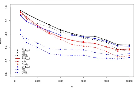
Figure 2.2 to 2.4 provide power results for µo = 375 under each of the three alternative
hypotheses. The power of the statistics with relatively lower performance are not displayed.
The statistics with fixed argument are only shown for the argumentdmax, which is the optimal
argument for the corresponding parameter setting. The display of the statistics with fixed
optimal argument is intended to show the best power performance of the collection of the
statistics with various argument settings, which is to be compared with the functional form of
0 2000 4000 6000 8000 10000 0.0 0.2 0.4 0.6 0.8 1.0
Power performance of statistics based on R~, R and C across σ under NS processes
σ P o w er ● ● ● ● ● ● ● ● ● ● ● ● ● ● ● ● ● ● ● ● ● ● ● ● ● ● ● ● ● ● ● ● ● ● ● ● R ~(
dmax) KSR~ CvMR~ R(dmax) KSR CvMR C(dmax) KSC CvMC
Figure 2.2: Power performance of statistics related to ¯R(d), ˜R(d), andC(d) under alternative hypothesis (1) with parameterµo =375.
Only maximum powers of ¯R(d), ˜R(d), andC(d) over values ofdconsidered are displayed;
0 2000 4000 6000 8000 10000 0.0 0.2 0.4 0.6 0.8 1.0
Power performance of statistics based on R~, R and C across σ under NS processes
σ P o w er ● ● ● ● ● ● ● ● ● ● ● ● ● ● ● ● ● ● ● ● ● ● ● ● ● ● ● ● ● ● ● ● ● ● ● ● R ~(
dmax) KSR~ CvMR~ R(dmax) KSR CvMR C(dmax) KSC CvMC
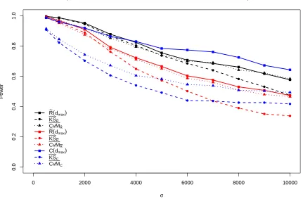
Figure 2.3: Power performance of statistics related to ¯R(d), ˜R(d), andC(d) under alternative hypothesis (2) with parameterµo =375.
Only maximum powers of ¯R(d), ˜R(d), andC(d) over values ofdconsidered are displayed;
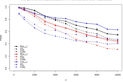
0 2000 4000 6000 8000 10000 0.0 0.2 0.4 0.6 0.8 1.0
Power performance of statistics based on R~, R and C across σ under NS processes
σ P o w er ● ● ● ● ● ● ● ● ● ● ● ● ● ● ● ● ● ● ● ● ● ● ● ● ● ● ● ● ● ● ● ● ● ● ● ● R ~(
dmax) KSR~ CvMR~ R(dmax) KSR CvMR C(dmax) KSC CvMC
Figure 2.4: Power performance of statistics related to ¯R(d), ˜R(d), andC(d) under alternative hypothesis (3) with parameterµo =375.
Only maximum powers of ¯R(d), ˜R(d), andC(d) over values ofdconsidered are displayed;
Under the alternative hypothesis (1), forµo =375, in general, the power of each test statistic
decreases asσincreases. The test statistics based on ˜R(d), ¯R(d) andC(d) generally have higher
powers than those based on Nmax(d) and Dmin(n). Figure 2.2 contrasts the power performance
of nine categories of statistics based on ˜R(d), ¯R(d) andC(d), including the statistics with fixed
arguments as well as their function forms. Among these nine, ˜R(d) has the highest power
and outperforms ¯R(d) andC(d) in all the settings of σ. The statistics related to ˜R(d) seem to
always outperform the statistics related to ¯R(d), which may be because ˜R(d) is more robust
and numerically more stable than ¯R(d). Among the six functional forms of statistics, CvM]R˜
andKSgR˜ outperform the other four functional forms of statistics, andCvM]R˜ has better power
performance thangKSR˜ asσincreases.
The power performance under alternatives (2) and (3) forµo = 375, available in Figure 2.3
and Figure 2.4, provide similar results to that described for alternative hypothesis (1). Power
is generally highest under alternative (2) and lowest under alternative (1) given all the other
settings remain constant. One noticeable difference from alternative hypotheses (2) and (3)
compared to (1) is that the powers ofC(d) outperform ˜R(d) whenσis not small. The
compari-son among the six functional forms of statistics shows similar results for alternative hypothesis
(1).
Forµo =1125, the powers of the test statistics are higher than whenµo =375. The powers
are closer to 1 and decrease less dramatically over σthan for the cases whereµo = 375. The
patterns of power comparisons are similar to the cases where µo = 375. Yet the powers of
˜
R(d) are comparable withC(d) whenσis large and both are quite close to 1 under alternative
hypotheses (2) and (3). The power performance of the statistics under the three alternative
hypotheses forµo =1125 is available in Figures A.1 to A.3 in Appendix A.
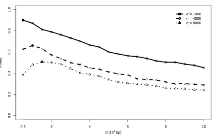
The power performance of ˜R(d) and C(d) seem to be best among the nine categories of
statistics, yet they suffer the disadvantage that they require a choice ofd. The optimal argument
choices of d are usually unknown in application. Moreover, the optimal choices of d may
0.0
0.2
0.4
0.6
0.8
1.0
Power performance of R~(d) under NS processes with selected paramters
P
o
w
er
● ●
● ●
● ●
● ●
● ●
● ●
● ● ● ●
● ● ● ●
●
0.5 2 4 6 8 10
●
σ = 1000
σ = 4000
σ = 8000
d (104bp)
Figure 2.5: Power performance of test statistics ˜R(d) across a grid ofdunder alternative hypothesis (1) with parameterµo =375.
In conclusion, the functional statistic CvM]R˜ is the preferred test statistic in applications
because it has the correct size and general high power performance, oftentimes close to the
best among all statistics; importantly, with this statistic no specific choice of tuning parameter
dneeds to be defined.
2.4
Application
2.4.1
Genotyping method
DNA was extracted from mouse tissue samples using the WizardR Genomic DNA Purification
Kit (Promega, Madison, WI). Isolated DNA was submitted to the London Regional Genomics
Centre to be processed (restriction enzyme digested, amplified, fragmented and fluorescently
labeled) and hybridized to the Mouse Diversity Genotyping Array (MDGA; AffymetrixR
,
Santa Clara, CA) [11]. Genotyping was performed for each of the three specific examples
within the context of separate experimental designs with a minimum cohort size of 12 samples
and a maximum of 351 samples. Genotyping Console (AffymetrixR
, Santa Clara, CA) was
used to call genotypes at the 493,290 SNP loci represented by the MDGA, using the
fluores-cence intensity data. The Genotyping Console software uses a clustering algorithm, Birdseed
v2, and assigns each SNP locus as 1 of 4 possible calls: AA (homozygous for the most
com-mon allele), AB (heterozygous, one of each allele), BB (homozygous for the less comcom-mon
allele), or no call if the SNP genotype calls did not cluster well with any of the three
possi-ble genotypes. The resulting data for each biological sample used for further analysis consist
of a list of SNP genotype calls, their locations in the genome (chromosome number and base
pair number) and the genotyping call given by Genotyping Console for each sample. In the
data sets utilized for testing for existence of clusters in this research, the events are defined as
SNP differences, which are the binary indicators of differences at SNP loci when contrasting
two biological samples. The genotyping call and the consequent SNP differences are putative
according to relevant national and international guidelines. Western University’s Animal Use
Subcommittee approved the study. All guidelines were followed including those approved
standard operating procedures for euthanasia.
2.4.2
Analyses for three biological samples of interest
Three specific examples are considered here.
1. Detection of known clusters of putative SNP differences in a mouse with a known mixed
genetic background;
2. Test for the existence of clusters of putative SNP differences arising postzygotically
be-tween two healthy tissues from a C57BL/6J mouse;
3. Test for the existence of clusters in comparison of two cancerous tissues from a
MMTV-PyMT transgenic mouse [25].
Rainfall plots portraying the mutation landscapes of the three samples are provided in
Fig-ure 2.6. On a rainfall plot, each point represents a single mutation with its distance (in base
pairs) to the previous mutation in log scale plotted on the y axis, and the base pair location in
the genome is plotted on the x axis. Rainfall plots display mutations detected along a single
chromosome or potentially across the entire genome. Although the plots offer a helpful
vi-sualization of the data including potential clustering, they do not provide formal evidence of