Available Online atwww.ijcsmc.com
International Journal of Computer Science and Mobile Computing
A Monthly Journal of Computer Science and Information Technology
ISSN 2320–088X
IMPACT FACTOR: 5.258IJCSMC, Vol. 5, Issue. 9, September 2016, pg.186 – 192
Image Compression Using Discrete
Cosine Transform Method
Qusay Kanaan Kadhim
Al-Yarmook University College / Computer Science Department, Iraq
ABSTRACT: The processing of digital images took a wide importance in the knowledge field in the last decades ago due to the rapid development in the communication techniques and the need to find and develop methods assist in enhancing and exploiting the image information. The field of digital images compression becomes an important field of digital images processing fields due to the need to exploit the available storage space as much as possible and reduce the time required to transmit the image.
Baseline JPEG Standard technique is used in compression of images with 8-bit color depth. Basically, this scheme consists of seven operations which are the sampling, the partitioning, the transform, the quantization, the entropy coding and Huffman coding. First, the sampling process is used to reduce the size of the image and the number bits required to represent it. Next, the partitioning process is applied to the image to get (8×8) image block. Then, the discrete cosine transform is used to transform the image block data from spatial domain to frequency domain to make the data easy to process. Later, the quantization process is applied to the transformed image block to remove the redundancies in the image block. Next, the conversion process is used to convert the quantized image block from (2D) array to (1D) vector. Then, the entropy coding is applied to convert the (1D) vector to intermediate form that is easy to compress. Finally, Huffman coding is used to convert the intermediate form to a string of bits that can be stored easily in a file which can be either stored on a storage device or transmitted to another computer. To reconstruct, the compressed image, the operations mentioned above are reversed.
Keywords: Image Compression, JPEG, Discrete Cosine Transform
1. INTRODUCTION
Image compression is an extremely important part of modern computing. By having the ability to compress images to a fraction of their original size, valuable (and expensive) disk space can be saved. In addition, transportation of images from one computer to another becomes easier and less time consuming (which is why compression has played such an important role in the development of the internet) [1].
algorithm reproduces the original exactly. A lossy algorithm, as its name implies, loses some data. Data loss may be unacceptable in many applications [8].
The JPEG image compression algorithm provides a very effective way to compress images with minimal loss in quality (lossy image compression method). Although the actual implementation of the JPEG algorithm is more difficult than other image formats and the compression of images is expensive computationally, the high compression ratios that can be routinely attained using the JPEG algorithm easily compensates for the amount of time spent implementing the algorithm and compressing an image [1].
Image compression has applications in transmission and storage of information. Image transmission applications are in broadcast television, remote sensing via satellite, military communications via aircraft, radar and sonar, teleconferencing, computer communications. Image storage applications are in education and business, documentation, medical image that arises in computer tomography, magnetic resonance imaging and digital radiology, motion pictures, satellite images weather maps, geological surveys and so on [12[.
Image files, especially raster images tend to be very large. It can be useful or necessary to compress them for ease of storage or delivery. However, while compression can save space or assist delivery, it can slow or delay the opening of the image, since it must be decompressed when displayed. Some forms of compression will also compromise the quality of the image. Today, compression has made a great impact on the storing of large volume of image data. Even hardware and software for compression and decompression are increasingly being made part of a computer platform [16].
2. Image Compression System Model
A typical image compression system is illustrated in figure (1). The original digital image is usually transformed into another domain, where it is highly de-correlated by the transform. This de-correlation concentrates the important image information into a more impact form. The compressor (encoder) then removes the redundancy in the transformed image and stores it into a compressed file or data stream. The decompressor (decoder) reverses this process to produce the recovered image. The recovered image may have lost some information, due to the compression, and may have an error or distortion compared to the original image [3].
Figure (1): A Typical Image Compression System
2.1 The Compressor
There are three basic parts to an image compressor, as shown in figure (2):
Figure (2): A General Image Compressor
2.1.1 Transform [17]
The discrete cosine transform (DCT) is a technique for converting a signal into elementary frequency components. The DCT was developed by Ahmed et al. (1974). The DCT is a close relative of the discrete Fourier transform (DFT). Its application to image compression was pioneered by Chen and Pratt in 1984.
• The One-Dimensional Discrete Cosine Transform
The discrete cosine transform of a list of n real numbers s(x), x=0… n-1, is the list of length n given by:
) 2 ) 1 2 ( cos( 1 0 ( ) ) ( 2 1 ) 2 ( ) ( n u x n
x s x
u C n u
S
for u=0… n-1 (1)
where
otherwise u for u C 1 0 2 1 2 ) (Each element of the transformed list S (u) is the inner product of the input list s(x) and a basis vector. The constant factors are chosen so that the basis vectors are orthogonal and normalized.
The list s(x) can be recovered from its transform S (u) by applying the inverse discrete cosine transform (IDCT): ) 2 ) 1 2 ( cos( 1
0 ( ) ( ) 2 1 ) 2 ( ) ( n u x n
u C u S u
n x
s
for x=0… n-1 (2)
where
otherwise u for u C 1 0 2 1 2 ) (Equation (2) expresses s as a linear combination of the basis vectors. The coefficients are the elements of the transform S, which may be regarded as reflecting the amount of each frequency present in the input s.
• The Two-Dimensional Discrete Cosine Transform
The one-dimensional DCT is useful in processing one-dimensional signals such as speech waveforms. For analysis of two-dimensional (2-D) signals such as images, a (2-D) version of the DCT is needed. For an n×m matrix s, the (2-D) of DCT is computed in a simple way.
The (1-D) of DCT is applied to each row of s and then to each column of the result. Thus, the transform of s is given by:
) 2 ) 1 2 ( cos( ) 2 ) 1 2 ( cos( 1 0 ( , ) 1 0 ) ( ) ( 2 1 ) 2 ( ) , ( m v x n u x m
y s x y
n x v C u C n v u S
for u=0… n-1,
v=0… m-1 (3) where
otherwise v u for v C u C 1 0 , 2 1 2 ) ( ), (Since the (2-D) of DCT can be computed by applying (1-D) transforms separately to the rows and columns, then the (2-D) of DCT is separable in the two dimensions.
The inverse discrete cosine transform (IDCT) for the two-dimensional DCT is: ) 2 ) 1 2 ( cos( ) 2 ) 1 2 ( cos( 1 0 ) , ( ) ( ) ( 1 0 2 1 ) 2 ( ) , ( m v x n u x m v v u S v C u C n u n y x
s
for x=0… n-1,
y=0… m-1 (4)
where
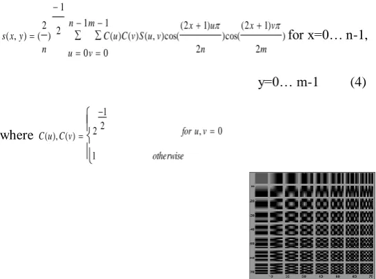
otherwise v u for v C u C 1 0 , 2 1 2 ) ( ), (Figure (3): The (8×8) array of basis images for the (2-D) DCT
2.1.2 Quantization
Quantization refers to the process of approximating the continuous set of values in the image data with a finite (preferably small) set of values [18]. Quantization is a necessary component in lossy coding and has a direct impact on the bit rate and the distortion of reconstructed images or videos [18]. The input to a quantizer is the original data, and the output is always one among a finite number of levels. The quantizer is a function whose set of output values are discrete, and usually finite. Obviously, this is a process of approximation, and a good quantizer is one which represents the original signal with minimum loss or distortion. There are two types of quantization:
• Linear Quantization [3]
Linear quantization is the most basic form of quantization. The transform coefficients are divided by a quantization step and the result is converted to an integer, by truncation of the decimal point as illustrated in equation (5):
i i qq
c
Integer
c
(5)where, qi is the quantization step,
ci is the transform coefficient,
and cq is the integer quantized coefficient.
The transform data is limited based on the 8 bit/pixel intensities of standard images. This allows a quantization step to be chosen, which limits the number of quantized states available, hence compressing the coefficients to a desired number of bits. However, it is not possible to control compression in this way, since a real system losslessly codes the quantized coefficients and this operation is not well defined.
It can be seen that equation (5) is not ideal and it can be improved to a more effective form,
i i qq
c
Integer
nearest
to
Round
c
(6)• Uniform Quantization [16]
The idea behind this quantization method is to release the range of the input set of data values into positive valued integers of, often, less width range. In this quantization method, the minimum MIN and the maximum MAX values of the input data must be specified, and then the input image of data is divided into a number of equidistant bins. The uniform quantization algorithm uses equally spaced bins it can, easily, found by equation (7):
(G 1)
MIN -MAX
MIN -y ) f(x, Roundoff y )
(x, Q
F (7)
where, Roundoff{x} approximates the enclosed x-value to nearest integer,
f(x, y) is the original input data,
FQ(x, y) their quantized value,
and G is the desired number of quantized level.
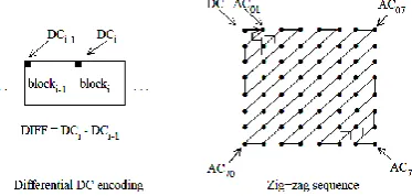
2.1.3 DC Coding and Zig-Zag Sequence
After quantization, the DC coefficient is treated separately from the 63 AC coefficients. The DC coefficient is a measure of the average value of the 64 image samples. Because there is usually strong correlation between the DC coefficients of adjacent 8x8 blocks, the quantized DC coefficient is encoded as the difference from the DC term of the previous block in the encoding order (defined in the following), as shown in Figure (4). This special treatment is worthwhile, as DC coefficients frequently contain a significant fraction of the total image energy.
Figure (4): Preparation of Quantized Coefficients for Entropy Coding
Finally, all of the quantized coefficients are ordered into the “zigzag” sequence, also shown in Figure (4). This ordering helps to facilitate entropy coding by placing low frequency coefficients (which are more likely to be nonzero) before high frequency coefficients.
2.1.4 Entropy Coding
The final DCT based encoder processing step is entropy coding. This step achieves additional compression losslessly by encoding the quantized DCT coefficients more compactly based on their statistical characteristics. The JPEG proposal specifies two entropy coding methods Huffman coding [8] and arithmetic coding [15]. The Baseline sequential codec uses Huffman coding, but codecs with both methods are specified for all modes of operation. It is useful to consider entropy coding as a 2step process. The first step converts the zigzag sequence of quantized coefficients into an intermediate sequence of symbols. The second step converts the symbols to a data stream in which the symbols no longer have externally identifiable boundaries. The form and definition of the intermediate symbols is dependent on both the DCT based mode of operation and the entropy coding method.
Huffman coding requires that one or more sets of Huffman code tables be specified by the application.
The same tables used to compress an image are needed to decompress it. Huffman tables may be predefined and used within an application as defaults, or computed specifically for a given image in an initial statistics gathering pass prior to compression. Such choices are the business of the applications which use JPEG; the JPEG proposal specifies no required Huffman tables.
conditioning tables can be used as inputs for slightly better efficiency, but this is not required.) Arithmetic coding has produced 510% better compression than Huffman for many of the images which JPEG members have tested. However, some feel it is more complex than Huffman coding for certain implementations, for example, the highest speed hardware implementations. (Throughout JPEG‟s history, “complexity” has proved to be most elusive as a practical metric for comparing compression methods.)
If the only difference between two JPEG codecs is the entropy coding method, transcoding between the two is possible by simply entropy decoding with one method and entropy recoding with the other.
2.1.5 Compression and Picture Quality
For color images with moderately complex scenes, all DCT based modes of operation typically produce the following levels of picture quality for the indicated ranges of compression. These levels are only a guideline quality and compression can vary significantly according to source image characteristics and scene content. (The units “bits/pixel” here mean the total number of bits in the compressed image including the chrominance components divided by the number of samples in the luminance component.)
•0.25-0.5 bits/pixel: moderate to good quality, sufficient for some applications; •0.5-0.75 bits/pixel: good to very good quality, sufficient for many applications; •0.75-1/5 bits/pixel: excellent quality, sufficient for most applications;
•1.5-2.0 bits/pixel: usually indistinguishable from the original, sufficient for the most demanding applications.
3. Baseline DCT Sequential Codec
The DCT sequential mode of operation consists of the FDCT and Quantization steps from section 2, addition to the Baseline sequential codec, other DCT sequential codecs are defined to accommodate the two different sample precisions (8 and 12 bits) and the two different types of entropy coding methods (Huffman and arithmetic).
Baseline sequential coding is for images with 8bit samples and uses Huffman coding only. It also differs from the other sequential DCT codecs in that its decoder can store only two sets of Huffman tables (one AC table and DC table per set). This restriction means that, for images with three or four interleaved components, at least one set of Huffman tables must be shared by two components. This restriction poses no limitation at all for interleaved components; a new set of tables can be loaded into the decoder before decompression of a non-interleaved component begins. For many applications which do need to interleave three color components, this restriction is hardly a limitation at all. Color spaces (YUV, CIELUV, CIELAB, and others) which represent the chromatic („„color‟‟) information in two components and the achromatic („„grayscale‟‟) information in a third are more efficient for compression than spaces like RGB.
One Huffman table set can be used for the achromatic component and one for the chrominance components. DCT coefficient statistics are similar for the chrominance components of most images, and one set of Huffman tables can encode both almost as optimally as two. The committee also felt that early availability of single-chip implementations at commodity prices would encourage early acceptance of the JPEG proposal in a variety of applications. In 1988 when Baseline sequential was defined, the committee‟s VLSI experts felt that current technology made the feasibility of crowding four sets of loadable Huffman tables in addition to four sets of Quantization tables onto a single commodity-priced codec chip a risky proposition. The FDCT, Quantization, DC differencing, and zigzag ordering processing steps for the Baseline sequential codec proceed just as described in section 2. Prior to entropy coding, there usually are few nonzero and many zero-valued coefficients. The task of entropy coding is to encode these few coefficients efficiently. The description of Baseline sequential entropy coding is given in two steps: conversion of the quantized DCT coefficients into an intermediate sequence of symbols and assignment of variable-length codes to the symbols.
4. Conclusions
The emerging JPEG continuous-tone image compression standard is not a panacea that will solve the myriad issues which must be addressed before digital images will be fully integrated within all the applications that will ultimately benefit from them. For example, if two applications cannot exchange uncompressed images because they use incompatible color spaces, aspect ratios, dimensions, etc. then a common compression method will not help.
References
1. Bibi Isac & V. Santhi, 2011 A Study on Digital Image and Video Watermarking Schemes using Neural Networks; International Journal of Computer Applications (0975 – 8887) Volume 12– No.9; 2011
2. Cox I, Miller M, Bloom J, Fridrich J, Kalker T , 2008 Digital Watermarking and Steganography Second Edition. Elsevier, 2008; ISBN 978-0-12-372585-1; Library of Congress Cataloging-in-Publication Data, Digital watermarking and steganography/Ingemar J. Cox ... [et al.].
3. I. Daubechies Basics of Wavelets; (Ten Lectures on wavelets; Orthonormal Bases of Compactly Supported Wavelets).
4. Bangxi Yu & Raj Jain, 2011 A Quick Glance at Digital Watermarking; Academic Project Report [www.cse.wustl.edu].
5. CSP Research and & Development, 2015 Embedding Interactive Data into an Audio-visual Content by Watermarking, [www.iitg.ernet.in]
6. Ingemar J. Cox, MatthewL.Miller, Jeffrey A. Bloom, Jessica Fridrich and Ton Kalker, Digital Watermarking and Steganography Second Edition; The Morgan Kaufmann Series in Multimedia Information and Systems Series Editor, Edward A. Fox, Virginia Poytechnic University; Elsevier.
7. Amara Graps, 1995 Introduction to Wavelets, IEEE Computational Science and Engineering, Summer 1995, vol. 2, num. 2, IEEE Computer Society, 10662 Los Vaqueros Circle, Los Alamitos, CA 90720, ©1995 8. Brani Vidakovic and Peter Mueller, 1991, Wavelets for Kids: A Tutorial Introduction; AMS Subject
Classification: 42A06, 41A05, 65D05.
9. Vaishali S. Jabade & Dr. Sachin R. Gengaje, 2011 Literature Review of Wavelet Based Digital Image Watermarking Techniques; International Journal of Computer Applications (0975 – 8887) Volume 31– No.1; 2011.
10.Yu-Ping Wang and Shi-Min Hu, A new watermarking method for 3D model based on integral invariant; Department of Computer Science and Technology, Tsinghua University.
11. Giorgos Louizis, Anastasios Tefas and Ioannis Pitas, 1999 Copyright Protection Of 3D Images Using watermarks Of Specific Spatial Structure; Department of Informatics, Aristotle University of Thessaloniki; Box 451, Thessaloniki 54006.
12.N. Nikolaidis!, I. Pitas, 1998 Robust image watermarking in the spatial domain; Elsevier, Signal Processing 66 (1998) 385Ð403; 0165-1684/98/$19.00 ( 1998 Elsevier Science B.V. All rights reserved. PII S0165-1684(98)00017-6
13.Dipti Prasad Mukherjee, Subhamoy Maitra, and Scott T., 2004 Spatial Domain Digital Watermarking of Multimedia Objects for Buyer Authentication; IEEE Transactions On Multimedia, Vol. 6, No. 1, February 2004
14.Jamal A. Hussein; 2010 Spatial Domain Watermarking Scheme for Colored Images Based on Log-average Luminance; Journal of Computing, Volume 2, Issue-1, 2010, ISSN 2151-9617 [Https://Sites.Google.Com/Site/Journalofcomputing/]
15.Pooja Dabas & Kavita Khanna, 2013 Efficient Performance of Transform Domain Digital Image Watermarking Technique over Spatial Domain; International Journal of Advanced Research in Computer Science and Software Engineering; Volume 3, Issue 6, 2013; ISSN: 2277 128X
16.Pooja Dabas & Kavita Khanna, 2013 A Study on Spatial and Transform Domain Watermarking Techniques;
International Journal of Computer Applications © 2013 by IJCA Journal, Volume 71 - Number 14 , Publication: 2013 Authors:, DOI: 10.5120/12429-9124
17.Kamran Hameed, Adeel Mumtaz, and S.A.M. Gilani, 2006 Digital Image Watermarking in the Wavelet Transform Domain; World Academic of Science, Engineering and Technology 13 2006
18.Jung-Hee Seo, and Hung-Bog Park, 2006 Data-Hiding Method using Digital Watermark in the Public Multimedia Network; International Journal of Information Processing Systems, Vol.2, No.2, June 2006; Copyright ⓒ 2006 KIPS (ISSN 1738-8899)