Eduardo Pareja-Tobes, Raquel Tobes
Oh no sequences! research group,Era7 Bioinformatics Plaza de Campo Verde, 3, 18001 Granada, Spain
September 16, 2019
Abstract Here we present
1. a model for amplicon sequencing
2. a definition of the best assignment of a read to a set of reference sequences
3. strategies and structures for indexing reference sequences and computing the best assign-ments of a set of reads efficiently, based on (ultra)metric spaces and their geometry The models, techniques, and ideas are particularly relevant to scenarios akin to 16S taxonomic profiling, where both the number of reference sequences and the read diversity is considerable.
Keywords bioinformatics, NGS, DNA sequencing, DNA sequence analysis, amplicons, ultrametric spaces, in-dexing.
1 Reads, Amplicons, References, Assignments
In this section we will define what we understand as reads, amplicons, references, and the best as-signment of a read with respect to a set of references.
In our model the reads are a product of the probability distribution for the 4 bases (A, C, G and T) in each position of the sequence.
Definition 1.0.1Read. A read𝑅 of length 𝑛 is a product∏𝑛−1𝑖=0 𝑅𝑖 of𝑛 probability distributions on
Σ = {𝐴, 𝑇 , 𝐶, 𝐺}. We will denote the length of a read as|𝑅|.
The corresponding probability mass function is thus defined on the spaceΣ𝑛 of sequences in Σ of length𝑛, thedomainof𝑅. The probability that𝑅assigns to a sequence𝑥 = (𝑥𝑖)𝑛−1𝑖=0 ∶ Σ𝑛is
𝑅(𝑥) =
𝑛−1
∏
𝑖=0
𝑅𝑖(𝑥𝑖)
Remark 1.0.2. The concrete finite alphabetΣis of course irrelevant in what follows; we will assume it being nucleotides as it is the one we find in DNA sequencing. The use of extended alphabets such as IUPAC codes covering combinations of bases is rendered superfluous by working with the read as a distribution, which can be evaluated in any𝑈 ⊆ Σ𝑛.
Defined as products of single-base distributions reas have positions both well-defined and indepen-dent. From the standard viewpoint of sequencing errors, read distribution positions are well defined if and only if indel errors are deemed impossible/highly unlikely; Their presence thus would force us to simply throw away all per-position quality information: we can no longer ascribe scores to posi-tions which are simply not well-defined. Fortunately, indel errors in Illumina sequencers¹have been considered as quite exceptional: in [11] it is reported that indel errors occur at rates of at most5 ∗ 10−6 per base.
All DNA sequencers output fastq: (sets of) sequences(𝑥𝑖, 𝑞𝑖)where the quality score𝑞𝑖 encodes
the probability of the base𝑥𝑖being correct². In the now standard Phred encoding a quality score𝑞 ∶ ℕ represents a probability oferror 𝑒 = 10−𝑞10.
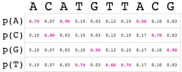
A generic read𝑅 is determined by|𝑅||Σ|values𝑝𝑖𝑗 in[0, 1]subject to the𝑛 equations∑𝑗𝑝𝑗𝑖 = 1. A Phred-encoded fastq read(𝑥𝑖, 𝑞𝑖)𝑛−1𝑖=0 though orresponds to a read∏𝑛−1𝑖=0 𝐷𝑖where the distribution
𝐷𝑖assigns probability1−𝑒𝑖to𝑥𝑖and𝑒3𝑖 to any of the other3bases;|𝑅|values and a sequence determine
¹the dominant platform by far, even more so in amplicon sequencing.
Figure 1: Read distribution derived from fastq
fastq reads. In what follows by a fastq read we will refer to a read for which there is a unique most likely base at each position, and the probabilities of any erroneous base -those different from the most likely one are all equal (see figure1).
Inside the sequencer all erroneous bases are not equally likely; fastq implies a considerable loss of information. But even putting that aside, it can be important in practice to allow for different error probabilities. For example, merging of the distributions corresponding to reads sequenced from the same molecule³becomes non-associative (and erroneous).
1.1 Amplicons
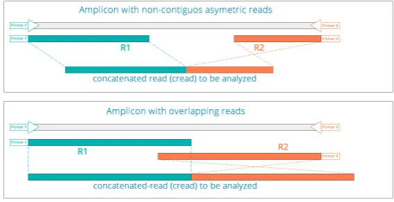
Amplicon sequencing in the Illumina platform normally produces two reads⁴, corresponding to sub-sequences of the target. Our model covers any type of amplicon, with overlapping or not overlapping reads, single or paired.
1.1.1 Extracting Amplicon-specific Fragments from References
An amplicon, loosely defined, corresponds to a set of primer pairs which would yield a pair of se-quenced reads (R1 and R2) from each target in the sample. These reads, viewed as products of prob-ability distributions onΣ, are isomorphic to a single read of length the sum of the amplicon reads lengths. If, as is normally the case, we have a collection of known complete target sequences⁵we simply need to produce the corresponding ampliconin-silico: extract the subsequences that would correspond to the sequenced fragments if the reference would be included in the sample. This will be further translated to the/an amplicon read along the permutation((𝑛1), ⋯ , (𝑛𝑘)) → (∑ 𝑛𝑖).
³such as what can be assumed to happen when using UMIs or equivalent mechanisms. ⁴Illumina single read sequencing, while possible, is not the standard.
1 Reads, Amplicons, References, Assignments
Figure 2: Non-overlapping vs overlapping amplicons
Paired-end amplicons whose reads are expected to overlap are analyzed by first merging the reads at those positions. We argue that the suposedly overlapping positions should be analyzed independently, as we do.
1. Amplicons normally have variable insert lengths, meaning that there is nosequence-independent way of determining which pairs of positions are supposed to come from the same nucleotide. 2. From the point of view of probability distributions this merging is commonly done wrong. Even
in [8] the result is only correct with respect to the most likely base.
If there are positions which actually come from the same nucleotide, these are given more weigth than the rest in the most likely reference. If this is not what we want, we should simply be sequencing amplicons whose reads don’t overlap⁶. In short, overlapping amplicon designs at the very best throw away sequence.
The reference sequences should be determined in terms of predicted primer binding sites, simulating sequencingin silico. Of course, as in any amplicon, the positions at which primers bind the target must be discarded; primers can and will bind even if a few bases differ, and what is sequenced is the primer sequence, not the target sequence.
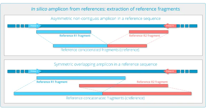
If the amplicon sequenced fragments are non-contiguous we simply need to extract the sequences that would be sequenced starting after each primer binding site. All these bases form a sequence on which we can evaluate our read qua product of distributions; that they could be separated by some other sequence or overlap in the target is irrelevant at this stage.
A reference thus is just a sequence which we expect can be obtained by sequencing an amplicon.
Figure 3: Reference extraction from target sequences
1.2 Alignment and Assignment
Definition 1.2.1Read Assignment. Given a read𝑅and a set𝒮 of sequences in the domain of𝑅, the *assignment* of𝑅in𝒮 is the subset𝐴(𝑅, 𝒮 ) ⊆ 𝒮 at which𝑅attains maximum probability.
𝒮 above is normally a proper subset ofΣ|𝑅|the domain of𝑅; if not, computing the corresponding as-signment trivializes: it simply corresponds to all possible combinations of maximums at each position (recall that𝑅is assumed to be a product of independent distributions).
An amplicon assignment algorithm is thus a process which has as input a set of readsℛ, and a set𝒮 of reference sequences, where reads and sequences are assumed to have the same length𝑛.
2 Assignment Strategies
For ease of exposition we will assume throughout that𝑅hasonemost likely sequence𝑚𝑅; the modifi-cations are minimal when that is not the case. Also, as is normally done, we will work with logarithms of probabilities. These we will callscores, so that our goal will be determining the best scoring refer-ences in𝒮.
If𝑚𝑅 ∈ 𝒮 then trivially𝐴(𝑅, 𝒮 ) = {𝑚𝑅}. But, even if it’s not,𝑚𝑅could be useful as a probe: intuitively 𝐴(𝑅, 𝒮 )should be “close” to𝑚𝑅, in some sense. We can make this idea precise through the
2 Assignment Strategies
2.1 Metric Bounds
Let’s see how the score of a reference𝑥 under𝑅 can be bounded both above and below in terms of 𝑑(𝑚𝑅, 𝑥).
Definition 2.1.1Worst, Best, Second Best Scores. For𝑅a read let
𝐵𝑅, 𝐵𝐸𝑅, 𝑊 𝐸𝑅∶ [0, |𝑅|[⊂ ℕ → ℝ
so that
• 𝐵𝑅(𝑖)is the best score of𝑅𝑖
• 𝐵𝐸𝑅(𝑖)is the second best score of𝑅𝑖(the best error) • 𝑊 𝐸𝑅(𝑖)is the worst score of𝑅𝑖(the worst error)
Example 2.1.2.
These functions just defined can be used to determine bounds for𝑅 on balls𝐵(𝑚𝑅, 𝑘)and co-balls
𝐹 (𝑚𝑅, 𝑘)with center𝑚𝑅. If𝑑(𝑚𝑅, 𝑥) ≤ 𝑘 at worst𝑥has𝑘mismatches with𝑚𝑅. The worst score we could possibly obtain with𝑘 mismatches is the sum of the𝑛 − 𝑘worst correct scores and the worst 𝑘errors. Dually, when𝑑(𝑚𝑅, 𝑥) ≥ 𝑘 at best x has again𝑘 mismatches with𝑚𝑅, and there could be no better way of picking them than (if possible) the best𝑛 − 𝑘 correct scores and the𝑘second best scores. We have just proved
Proposition 2.1.3. For𝑅a read of length𝑛
𝑅𝐵(𝑚
𝑅,𝑘)≤ 𝑈 (𝑘) 𝑅𝐹 (𝑚
𝑅,𝑘)≥ 𝐿(𝑘)
(1)
where
𝑈 (𝑘) = ∑ max𝑛−𝑘𝐵𝑅+ ∑ max𝑘𝑊 𝐸𝑅
𝐿(𝑘) = ∑ min𝑛−𝑘𝐵𝑅 + ∑ min𝑘𝐵𝐸𝑅
(2)
Remark 2.1.4. Note that for a generic𝑅 these bounds (taking as domain of𝑅 all possible reference sequences) are not tight; the worst correct score and the worst error (for example) could correspond to the same𝑅𝑖, thus being impossible to attain. They are tight though when𝑅is of fastq type, as
is easily seen by induction on the length of the sequence.
Trivially𝑘 < 𝜆(𝑘), and once we have found 𝑥 ∶ 𝒮 with𝑑(𝑚𝑅, 𝑥) = 𝑘 our bounds imply that it is
strictly better than any𝑥′∶ 𝒮 for which𝑑(𝑚𝑅, 𝑥′) ≥ 𝜆(𝑘):
Proposition 2.1.6. Let𝑥be a reference,𝑘 = 𝑑(𝑚𝑅, 𝑥). Then the assignment is contained in𝐵(𝑚𝑅, 𝜆(𝑘)).
Proof. As by hypothesis the open ball is nonempty, it is enough to prove that𝑅(𝑥) < 𝑅𝐹 (𝑚
𝑅,𝜆(𝑘)). But from the definition of𝜆(𝑘)and2.1.3
𝑅(𝑥) ≤ 𝑈 (𝑘) < 𝐿(𝜆(𝑘)) ≤ 𝑅 𝐹 (𝑚 𝑅,𝜆(𝑘))
Computationally this result is as advantageous as calculating𝑑(𝑚𝑅, 𝑥)is with respect to evaluating
𝑅(𝑥). But we are in a metric space, and the triangular inequality gives us (once we compute a distance 𝑑(𝑚𝑅, 𝑥)) a ball containing the assignment definedonlyin terms of the reference set and the read:
Corollary 2.1.7. Under the hypotheses of2.1.6the assignment is contained in the ball𝐵(𝑥, 𝑘 + 𝜆(𝑘)).
Proof. Obvious (triangular inequality).
These results restrict the domain of our search once we compute a distance𝑑(𝑚𝑅, 𝑥). But the𝑈 , 𝐿 bounds can also be used to discard whole balls once we have a𝑥′far enough from𝑚𝑋 relative to a
previously inspected𝑥.
Proposition 2.1.8. Let𝑥 ∶ 𝒮 , 𝑘 = 𝑑(𝑚, 𝑥). Then for any𝑥′∶ 𝒮 such that𝑘′= 𝑑(𝑚, 𝑥′) > 𝜆(𝑘)
𝑅𝐵(𝑥′,𝑘′−𝜆(𝑘))> 𝑅(𝑥)
Proof. The ball𝐵(𝑥′, 𝑘′− 𝜆(𝑘))is contained in𝐹 (𝑚, 𝜆(𝑘))and thus2.1.6applies.
All this already points to a possible index structure: the balls𝐵(𝑥, 𝑘 + 𝜆(𝑘)), 𝐵(𝑥′, 𝑘′− 𝜆(𝑘))are all intrinsic to the reference set, and𝜆(𝑘)is easy to compute⁷. The complexity of the resulting structure looks daunting though. Checking containment for two balls𝐵(𝑥, 𝑘), 𝐵(𝑥′, 𝑘′) potentially requires computing all the relevant distances, the intersection of two balls is not a ball that would require somethingmore than mere balls.
What we do instead is freely build a new metric space out of𝒮 ⊂ (Σ𝑛, 𝑑)on which the balls are as easy to manage as one could possibly hope.
2 Assignment Strategies
2.2 Free Ultrametrics as Indexes
Definition 2.2.1Ultrametric Space. An ultrametric space is a metric space(𝑋 , 𝑑)for which
𝑑(𝑥, 𝑧) ≤ max{𝑑(𝑥, 𝑦), 𝑑(𝑦, 𝑧)}
See [15, 12, 6, 14, 9,7] for references on ultrametric spaces. What interests us about them is the particularly simple structure of the poset of balls:
Proposition 2.2.2. In an ultrametric space
• 𝑥′∈ 𝐵(𝑥, 𝜆) ⇒ 𝐵(𝑥, 𝜆) = 𝐵(𝑥′, 𝜆)
• 𝐵(𝑥, 𝜆) ∩ 𝐵(𝑥′, 𝜆′)is either empty or the one with minimum radius
In particular, two balls are either disjoint or one is contained in the other. It follows that for a fixed 𝜆the balls𝐵(𝑥, 𝜆)are equivalence classes for the relation𝑥 ∼ 𝑦 whenever𝑑(𝑥, 𝑦) ≤ 𝜆: transitivity follows from 1. above. The poset of balls is thus a tree where leaves are the points.
From now on we will refer to balls in an ultrametric space asclusters, and denote them as𝐶(𝑥, 𝜆).
Definition 2.2.3Lower/Upper Radius, Point Radius. The lower radius of a cluster𝐶(𝑥, 𝜆)is the mini-mum𝜆′for which𝐶(𝑥, 𝜆′) = 𝐶(𝑥, 𝜆′); the upper radius is the maximum onesuch. The point radius of 𝑥 ∶ (𝑋 , 𝑑)in an ultrametric space is𝑝(𝑥) = sup { 𝜆 ∶ 𝐶(𝑥, 𝜆) = {𝑥} }.
Definition 2.2.4Cluster-compatible Order. A cluster-compatible order is anylinear order ≤on the points of(𝑋 , 𝑑)for which every cluster is an interval:
𝐶(𝑥, 𝜆) = [𝑠(𝑥, 𝜆), 𝑒(𝑥, 𝜆)[
and for which cluster intersection corresponds to interval intersection
𝐶(𝑥, 𝜆) ∩ 𝐶(𝑥′, 𝜆′) = [max(𝑠(𝑥, 𝜆), 𝑠(𝑥′, 𝜆′)), min(𝑒(𝑥, 𝜆), 𝑒(𝑥, 𝜆′))[
Proposition 2.2.5. Any ultrametric space admits a cluster-compatible order.
Proof. There’s a maximum radius 𝜆0 at which 𝑋 ≠ 𝐶(𝑥, 𝜆0). Pick a linear order on the clusters
{𝐶(𝑥, 𝜆0)∶ 𝑥 ∶ 𝑋 }, and proceed recursively on each. Points correspond to the clusters 𝐶(𝑥, 𝑝(𝜆)),
Note that in the proof above we can pickanylinear order on clusters of the same radius.
We can then storeall balls in an ultrametric space as intervals, and thus store points in any linear data structure (arrays) so that points get closer as we reduce intervals centered at any point. How many of such intervals, though? It turns out that an ultrametric space𝑋 , 𝑑has at most2|𝑋 |different clusters.
Proposition 2.2.6. For(𝑋 , 𝑑)an ultrametric space the image of𝑑 has cardinality at most|𝑋 | − 1.
Proof. Induction on|𝑋 |.
Proposition 2.2.7. [13] There are at most2|𝑋 |balls in an ultrametric space.
Proof. Again induction on|𝑋 |.
2.2.1 Free Ultrametric Spaces
We have just seen that the structure of balls in an ultrametric space is particularly simple:
1. There are at most2|𝑋 |different clusters 2. The inclusion relation is a tree order
3. This order admits linear order extensions under which clusters are intervals in an intersection-preserving way
Being ultrametric though can be seen as apropertythat a metric space might satisfy –or not, as is the case of(Σ𝑛, 𝑑𝐻). What we can try to construct is the best possible generic approximation of a metric
space by an ultrametric one: aleftadjoint𝐶 ∶Met→UMetto the inclusionUMet→Met. The unit𝜂∶ 𝐼 𝑑 → 𝐶𝑈 (𝑋 )yields at each metric space(𝑋 , 𝑑)a morphism inMet𝜂𝑋∶ 𝑋 → 𝐶(𝑋 ).
Proposition 2.2.8. The free ultrametric space exists and is given by the same set of points and distance
𝑑𝐶𝑋(𝑥, 𝑦) = inf { max {𝑑𝑋(𝑥𝑖, 𝑥𝑖+1)∶ (𝑥 = 𝑥0, … , 𝑥𝑛= 𝑦)} }
Proof. 𝐶 as defined is clearly a functor, the identity on points the components of a natural transfor-mation𝐼 𝑑 → 𝑈 𝐶, and the unit-counit equations are trivial to verify. There is also a totally straight-forward proof establishing the standard bijection between morphisms𝐶𝑋 → 𝐿and𝑋 → 𝐿.
As the right adjoint is fully faithful𝐶(𝑋 ) ≅ 𝑋for any ultrametric space𝑋. By construction𝜂𝑋∶ 𝑋 →
𝐶𝑋is essentially surjective on objects; it is further guaranteed to be injective on objects in our main case of interest:
Proposition 2.2.9. If(𝑋 , 𝑑)is a finite metric space then the unit at𝑋:𝜂𝑋∶ 𝑋 → 𝐶𝑋 is the identity on objects.
2 Assignment Strategies
Remark 2.2.10. Having a morphism𝜂 ≡ 𝜂𝑋∶ 𝑋 → 𝐶𝑋implies that𝑑(𝑥, 𝑦) ≥ 𝑑𝐶𝑋(𝜂(𝑥), 𝜂(𝑦)). If𝜂is
bijective on objects we can think of𝑑𝐶𝑋 as a distance on the same set points which is allowed to get points closer, but not set them farther than they were. As a consequence
Lemma 2.2.11. 𝐵(𝑥, 𝜆) ⊆ 𝐶(𝑥, 𝜆).
2.2.2 Clusters and Assignments
We wanted to use clusters in𝐶(𝒮 )as a sort of substitute for balls in𝒮; let’s see how what we know about bounding and discarding references for assignment relates with these clusters.
Just for future reference let’s record the obvious
Proposition 2.2.12. Let𝑥 ∶ 𝒮 , 𝑘 = 𝑑(𝑚, 𝑥).
Then the assignment is in any cluster𝐶(𝑥, 𝑘′) ⊆ 𝐵(𝑥, 𝑘 + 𝜆(𝑘)).
Proposition 2.2.13. Let𝑥, 𝑥′∶ 𝒮 such that𝑘′ = 𝑑(𝑚, 𝑥′) > 𝜆(𝑘).
Then we can discard any cluster𝐶(𝑥′, 𝑘″) ⊆ 𝐵(𝑥, 𝑘′− 𝜆(𝑘)).
With respect to bounding2.2.11and2.1.7yield
Corollary 2.2.14. Let𝑥be a reference,𝑘 = 𝑑(𝑚, 𝑥). Then the assignment is contained in𝐶(𝑥, 𝑘 + 𝜆(𝑘)).
For discarding though we don’t have any generic way of determining when𝐶(𝑥′, 𝜆′) ⊆ 𝐵(𝑥, 𝜆).
2.2.3 Radii
We will stop now and look at different radii on subsets of metric spaces; these and derived notions will be used to bound/discard clusters later on.
Definition 2.2.15 inner/outer radii. Let 𝑥 ∶ (𝑋 , 𝑑). The inner, outer radii at 𝑥 are the maps 𝑖𝑥, 𝑜𝑥∶ 𝑃(𝑋 ) → 𝑅defined by
𝑖𝑥(𝑈 ) = sup { 𝜆 ∶ 𝐵(𝑥, 𝜆) ⊆ 𝑈 }
𝑜𝑥(𝑈 ) = inf { 𝜆 ∶ 𝑈 ⊆ 𝐵(𝑥, 𝜆) }
(3)
When allowing any basepoint we have the inner, outer radii𝑖, 𝑟 ∶ 𝑃(𝑋 ) → 𝑅
𝑖(𝑈 ) = sup { 𝑖𝑥(𝑈 )∶ 𝑥 ∶ 𝑈 }
𝑜(𝑈 ) = inf { 𝑜𝑥(𝑈 )∶ 𝑥 ∶ 𝑈 }
(4)
Proposition 2.2.16. Let𝑈 ∶ 𝑃(𝑋 )a subset of the metric space𝑋,𝑥 ∶ 𝑈. Then
𝐵(𝑥, 𝜆) ⊆ 𝑈 ⟺ 𝜆 ≤ 𝑖𝑥𝑈 (5)
𝑈 ⊆ 𝐵(𝑥, 𝜆) ⟺ 𝑜𝑥𝑈 ≤ 𝜆 (6)
Proof. Trivial.
Definition 2.2.17Entometer, Diameter. The entometer, diameterentom(𝑈 ), diam(𝑈 )of a subset𝑈 ⊆ (𝑋 , 𝑑)are
entom(𝑈 ) = inf { 𝑖𝑥(𝑈 )∶ 𝑥 ∶ 𝑈 }
diam(𝑈 ) = sup { 𝑜𝑥(𝑈 )∶ 𝑥 ∶ 𝑈 }
(7)
Remark 2.2.18. entom(𝑈 ) is the minimum distance between𝑈 and its complementary 𝑈∗, which implies thatentom(𝑈 ) = entom(𝑈∗).
Proposition 2.2.19. Let𝑈 ∶ 𝑃(𝑋 )be a subset of the metric space𝑋. Then
∀𝑥 ∶ 𝑈 𝐵(𝑥, 𝜆) ⊆ 𝑈 ⟺ 𝜆 ≤ entom 𝐴 (8)
∀𝑥 ∶ 𝑈 𝑈 ⊆ 𝐵(𝑥, 𝜆) ⟺ diam 𝐴 ≤ 𝜆 (9)
Proof. Trivial.
For reference
Lemma 2.2.20. Let𝑈 ∶ 𝑃(𝑋 ), 𝑥 ∶ 𝑈. Then
entom 𝑈 ≤ 𝑖𝑥𝑈 ≤ 𝑖𝑈 (10)
𝑜𝑈 ≤ 𝑜𝑥𝑈 ≤ diam 𝑈 (11)
Proof. Trivial.
Remark 2.2.21. Somewhat contrary to intuition, there is no generic relationship between inner and outer radii, or entometers and diameters. It is easy to find examples where𝑖𝑥𝑈 ≤ 𝑜𝑥𝑈 and𝑜𝑥′𝑈 ≤ 𝑖𝑥′𝑈. We do have though
2 Assignment Strategies
2.2.4 Cluster Radii, Bounding, Discarding
Let’s see what we can say about the radii of clusters when seen as subsets of the original space (𝑋 , 𝑑).
Lemma 2.2.23. Let𝜆be the upper radius of a cluster𝐶 = 𝐶(𝑥, 𝜆). Then as a subset of the original metric spaceentom 𝐶 = 𝜆.
Proof. Quasi-obvious.
In particular for a cluster𝜆 ≤ entom 𝐶(𝑥, 𝜆). What about the inner radius? For any point𝑥′∶ 𝐶 = 𝐶(𝑥, 𝜆)we have that𝜆 ≤ 𝑖𝑥′𝐶so we can only say that𝜆 ≤ 𝑖𝐶.
In the context of our problem the inner radius at a point can be used to determine clusters which are known to contain the assignment:
Proposition 2.2.24. Let𝑥be a reference,𝑘 = 𝑑(𝑚, 𝑥). Then the assignment is contained in any cluster 𝐶(𝑥, 𝑘′)for which𝑘 + 𝜆(𝑘) ≤ 𝑖𝑥(𝐶(𝑥, 𝑘′)).
Obviously, once we have computed𝑑(𝑚, 𝑥), bounding through the inner radius at⁸𝑥 will consist in determining thesmallestcluster𝐶containing𝑥for which𝑘 + 𝜆(𝑘) ≤ 𝑖𝑥𝐶.
The entometer plays the same role, with the difference that there is no dependence on the particular reference, only the clusters containing it:
Proposition 2.2.25. Let𝑥be a reference,𝑘 = 𝑑(𝑚, 𝑥). Then the assignment is contained in any cluster 𝐶containing𝑥for which𝑘 + 𝜆(𝑘) ≤ entom 𝐶.
As remarked before, we will always refer to thesmallestsuch cluster when bounding by the entome-ter.
The situation when discarding clusters is of course dual. In the standard context for discarding a reference we have
Proposition 2.2.26. Under the hypotheses of2.2.13we can discard any cluster𝐶containing𝑥′for which 𝑜𝑥′𝐶 ≤ 𝑘′− 𝜆(𝑘).
And here when discarding by the outer radius at𝑥′we will always find thebiggestcluster satisfying the above.
The version without reference on the cluster side involves of course the diameter:
Proposition 2.2.27. Under the hypotheses of2.2.13we can discard any cluster𝐶containing𝑥′for which diam 𝐶 ≤ 𝑘′− 𝜆(𝑘).
2.3 Probability Thresholds
In most cases we would like to establish a lower? bound𝑠0 for assignment probabilities, treating as
unassigned the resulting reads. For this we can first determine a minimum distance from𝑚𝑅threshold
𝐾 for which𝑑(𝑚𝑅, 𝑥) > 𝐾 ⟹ 𝑅(𝑥) > 𝑠0. As in2.2.26we can discard whole clusters in terms of their outer radius
Proposition 2.3.1. If𝑑(𝑚𝑅, 𝑥) = 𝑘 > 𝑀 where𝑀 is some minimum distance threshold, we can discard
any cluster𝐶(𝑥, 𝑘)for which
𝑜𝑥(𝐶(𝑥, 𝑘′)) ≤ 𝑘 − 𝑀
3 Implementation Strategies
3.1 Indexing
Given(𝑋 , 𝑑)a metric space, the set of all clusters (balls in the free ultrametric space), possibly au-mented with further data at each cluster/point, will be called from now on anultrametric indexon𝑋. The sort of extra data we will consider consists in inner/outer radii and the corresponding centers, and entometers/diameters. As with any index, there’s a speed/space tradeoff; hardware limitations and any generic information about the sort of input this index will be queried with should guide the decision on which extra data the index should contain.
From what we saw in the previous sections, inner radii and entometers can be used tobound the search to a cluster, while outer radii and diameters todiscard clusters. If we expect our queries to be diverse (each one close to far away reference points) we will spend much more time discarding than bounding our search; we could then add outer centers and their radii to all clusters, or simply entometers (just one number per cluster).
As for the points themselves, different storage layouts are available, each one more suitable to a certain sort of queries. For example, using anycluster-compatible order, the points themselves can be stored in a flat array, while clusters are sets of nested intervals over this array. These intervals can be stored using variants of segment trees, or using an Elias-Fano encoding of the start and end points. Another possibility lies in simply keeping the list of nested clusters at each point, and then compress those lists using incremental compression. These sort of structures will perform really good if the whole index can be fit in memory.
3 Implementation Strategies
In any case, when using clusters as an index there are two extremes
• Store the inner/outer radii foreachpoint of every cluster • Compute just theentomanddiamof each cluster
Storingall𝑖𝑥, 𝑜𝑥radii for each cluster requires𝑂(2𝑛 log(𝑛))space, while the cost ofdiamandentomis
negligible. In terms of computation, bothdiamandentomcan be computed without much extra cost while we build the clusters; computing all inner/outer radii is bound to be considerably expensive.
3.1.1 Index Computation
Computing the cluster of radius𝜆containing a given point reduces to computing a transitive closure; not much can be said without assuming something about the metric at hand. A straightforward algorithm consists in starting with𝑈 = 𝐵(𝑥, 𝜆), then for each𝑥′∈ 𝑈 compute the corresponding ball 𝐵(𝑥′, 𝜆)and add those not in𝑈; now do the same with the newly added points until we reach a fixed point.
In cases where the distance has a discrete range (like in our main case of interest, Hamming distance between strings of the same length) we can compute in parallel all clusters for each possible distance value; the inclusion order can be trivially computed afterwards. We can also follow either a bottom-up or top-down approach, where in the first case clusters get joined to form clusters of bigger radii, while in the second one we can restrict the ambient space to a cluster of a bigger radius.
3.2 Standard Amplicon Situation
We will now outline how a full sequence assignment process for an amplicon where
1. The reference set will be reused across several experiments, and thus it makes sense to index it 2. The number ofdifferent sequence assignments is small when compared with the number of
reads
3. Most reads will be close to some point in the reference
These requirements are satisfied by all the standard amplicons used for taxonomic profiling: 16S for prokaryotes, 18S, mithochondrial 16S, or ITS for eukaryotes, etc.
3.2.1 Find Exact Assignments
First, we compute those reads which haveexactassignments: a reference equal to the read most likely sequence. A simple hash set will suffice, given that reference databases have on the order of millions of sequences. As output we get a set of references seen, sorted from more to less reads assigned to it.
3.2.2 Assign Inexactly or Discard
The rest of the reads will then be either unassigned or inexactly assigned, meaning that their most likely sequence is not part of the reference. We can obtain a metric bound M from the user-provided probability threshold for unassignment using the probability bounds2.1.3for each read and2.3.1. The ultrametric index we will use has extra data for clusters their outer centers, outer radii, and inner radii of outer centers.
Two distinct processes are followed for discarding and assigning a read.
For discarding, we traverse an ultrametric index which stores for each cluster its outer center and corresponding radius. All the clusters in a level of this tree constitute a partition of the whole space; thus if the read can be discarded based on the metric bound M, there will be a level at which all clus-ters can be discarded metrically using the distance of the read with the corresponding outer center⁹. Computing the distances with all outer centers per level, we either
• can discard all clusters and thus the read
• the read is assignable after comparing with an outer center
Note that whenever we cannot metrically assign/discard with respect to a center (the distance lies in between the corresponding bounds) we evaluate the corresponding probability directly. In this and in all other probability computations, we actually compute the mismatches count and a bit vector with their positions (between the most likely sequence and the reference), and the maximum probability of the read¹⁰. From this data we can thus compute those indexes at which they differ¹¹and substract (in log space) the corresponding probabilities.
For assigning we simply compute the distances of the most likely sequence with the outer centers, bounding and discarding at each level. As when discarding, whenever metric bounds are uninforma-tive we compute probabilities explicitly.
⁹at worst, at the point where all clusters are singletons ¹⁰This is trivial for fastq input.
4 Related Work
3.2.3 One Pass Alternative
While the implementation does two passes over the input, it can be run online with minimal modifi-cations. The two-pass implementation is chosen as default based on the assumption that most reads without exact assignments are similar to one of those which have them; this will be so if some of those differences are caused by sequencing errors with respect to those with exact ones.
4 Related Work
Finding the best assignment as we have defined bears a strong resemblance with the classical nearest neighbour problem [4,3], for which there exist several relevant indexing strategies [1,2,10]. It would be interesting to compare the use of the free ultrametric space here with those index structures; in this area ultrametrics appear in [5]. Tropashko [16] is also relevant with respect to tree indexes.
References
[1] A compact space decomposition for effective metric indexing
Edgar Chávez and Gonzalo Navarro
Pattern Recognition Letters26(9): (2005), 1363–1376.
[2] An effective clustering algorithm to index high dimensional metric spaces
Edgar Chávez and Gonzalo Navarro
Proceedings Seventh International Symposium on String Processing and Information Retrieval. SPIRE 2000 IEEE 2000, 75–86.
[3] Searching in metric spaces
Edgar Chávez, Gonzalo Navarro, Ricardo Baeza-Yates, and José Luis Marroquín ACM computing surveys (CSUR)33(3): (2001), 273–321.
[4] Nearest neighbor queries in metric spaces
Kenneth L Clarkson
Discrete & Computational Geometry22(1): (1999), 63–93.
[5] Fast, Linear Time Hierarchical Clustering using the Baire Metric
Pedro Contreras and Fionn Murtagh
Journal of Classification29(2 2012), 118–143. DOI:10.1007/s00357-012-9106-3. [6] Finite Ultrametric Balls
O. Dovgoshey (October 2018) eprint:1810.03128v1 URL:http://arxiv.org/abs/1810.03128v1.
[7] Extremal properties and morphisms of finite ultrametric spaces and their representing trees
[8] Error filtering, pair assembly and error correction for next-generation sequencing reads
Robert C. Edgar and Henrik Flyvbjerg Bioinformatics31(21 2015), 3476–3482. DOI:10.1093/bioinformatics/btv401.
[9] Spectral decomposition of ultrametric spaces and topos theory
Alex J Lemin
Topology Proc26(2): 2002, 721–739.
[10] Recursive lists of clusters: A dynamic data structure for range queries in metric spaces
Margarida Mamede
International Symposium on Computer and Information SciencesSpringer 2005, 843–853. [11] Illumina error profiles: resolving fine-scale variation in metagenomic sequencing data
Melanie Schirmer, Rosalinda D’Amore, Umer Z. Ijaz, Neil Hall, and Christopher Quince BMC Bioinformatics17(1 2016)
DOI:10.1186/s12859-016-0976-y. [12] Dissimilarities, Metrics, and Ultrametrics
Dan A. Simovici (2019).
[13] Multivalued and Binary Ultrametrics, and Clusterings
Dan A. Simovici misc Iasi, Romania, 2014
URL:https://www.cs.umb.edu/~sim/sIASI.pdf. [14] Several remarks on dissimilarities and ultrametrics
Dan A Simovici
Scientific Annals of Computer Science25(1): (2015), 155. [15] Mathematical tools for data mining
Dan A Simovici and Chabane Djeraba SpringerVerlag, London(2008).
[16] Nested intervals tree encoding in SQL
Vadim Tropashko