International Journal of Advanced Research in Computer Science
RESEARCH PAPER
Available Online at www.ijarcs.info
© 2015-19, IJARCS All Rights Reserved 42
Simulation to Demonstrate Traffic Junction Management
Aniket Acharya
Department Of Computer Engineering Thakur College Of Engineering And Technology
Mumbai, India
Rabab Kazi
Department Of Computer Engineering Thakur College Of Engineering And Technology
Mumbai, India
Anish Narkar
Department Of Computer Engineering Thakur College Of Engineering And Technology
Mumbai, India
Harshala Yadav
Department Of Computer Engineering Thakur College Of Engineering And Technology
Mumbai, India
Abstract: In recent years due to an increase in the number of vehicles and limited growth in infrastructure there has been a rise in congestion of
traffic especially in metropolitan cities. The project discusses various algorithms which can be implemented in various scenarios to dynamically determine green times and phase sequence of traffic light and reduce congestion in cities. To confirm the validity of the algorithms some case studies are considered and simulations have been performed to determine the effects of adopting the mentioned algorithms. The proposed system tries to incorporate all the functionalities of the existing systems in order to create a hybrid system, which would ensure that the current traffic scenario is improved by the proposed algorithm to optimize the flow of traffic, creating a smooth passage for services, which are time sensitive. Provisions are proposed to deal with fluctuating nature of urban traffic, dealing with emergencies, incident and other such factors .We aim to create a simulation of a traffic model with the current and proposed scenarios to study the impacts of the proposed algorithm.
Keywords: Traffic junction algorithm, traffic congestion, traffic control, dynamic traffic management, traffic management system, traffic simulation, SUMO
I. INTRODUCTION
The population of motorized vehicles has experienced a 100-fold increase since the 1990’s; however, the expansion in the road network has not been proportional with this increase. While the motor vehicle population has risen from 0.3 million to over 30 million over a course of 50 years [5], the road network has only expanded by 3.3 million km during the same period. This disparity is one of the major causes of increase in traffic congestion across all the major cities. There are numerous approaches to resolve the issue of traffic congestion for which the solutions range from using efficient cars to increasing the infrastructure. However, these approaches are constrained by time and other resources. We propose a more feasible solution - to modify the current traffic management systems.
The proposed project is a dynamic traffic management system. This system uses a specially developed algorithm to dynamically adjust the green time for each signal so as to optimize the flow of traffic to minimize traffic jams and ensure free flow of traffic in all directions. The system allocates green time to each road according to the traffic on that road. This means that more the traffic on a road, greater the green time allocated. Of course, the term “more traffic” is relative to traffic on other roads that link to that junction. There are threshold levels for maximum and minimum green time so that no road is kept waiting for too long as this could create more traffic than it clears. It should be noted that the cycle time for high traffic scenarios is fixed. This concept is explained in detail in the algorithm.
The algorithm designed was compared to a few other algorithms including the static algorithm that is currently used at traffic signals and the benefits were quantified and expressed in terms of time saved and fuel saved.
II. LITERATURE REVIEW
A. Smart Traffic Light Junction Management
An algorithm has been implemented for the dynamic management of intersections that uses data collected by the wireless sensor networks (WSN) to determine the phase sequence and the green times duration. The results are indicative of the fact that, the implemented algorithm facilitates the betterment of the management of traffic light junctions. Also, the algorithm is suitable for intersections affected by irregular traffic flows varying throughout the day.[1], [3].
1) Algorithm
The algorithm processes the data and determines the phase sequences and the green times of each phase. The algorithm uses the number of vehicles to determine different parameters like the length of the queue for different lanes. The results obtained from the algorithm are then input to The Traffic Lights Control module which uses the information to manage the sequence and the duration of traffic lights.
Rabab Kazi et al, International Journal of Advanced Research in Computer Science, 7 (2), March- April, 2016,42-48
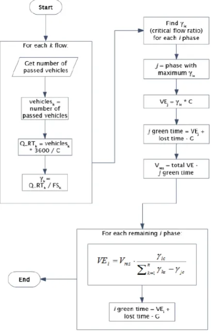
queue length for each flow (input variable) to assign a priority to each phase equivalent to the maximum queue length of that phase. The phase sequence is then determined by sorting it in decreasing order of priority. In the second step, the green times are calculated. Figure 1 presents the flowchart for the calculation of green times. For each flow, the algorithm obtains the number of vehicles that passed during the previous traffic light cycle and using this value determines the current traffic volume (Q RT).
Figure 1. Flow chart to determine green time-Base Paper
The algorithm then recalculates the next traffic cycle’s green time duration using the obtained value. The flow ratio di for every flow i is given as the ratio between the volume of traffic Q and the saturation flow rate FS:
di = Qi / FSi (1)
The data intercepted by the wireless sensors is used by the algorithm to recalculate the incoming stream at every traffic light cycle. For each lane, the number of vehicles passed in each cycle is counted. This data is converted in vehicles/h and subsequently used to recalculate the flow ratio for each traffic flow. For each phase, the critical lane (the one with a higher flow ratio) is established. The phase with the highest flow ratio is found; to this j-phase we assign a saturation flow ratio equal to 1, giving rests to the remaining phases in proportion to their flow ratios
V Ej /C =di (2)
Where V Ej is the effective green time for the j-phase and C is the traffic light cycle duration. Once V Ej is obtained, it is possible to calculate the j-phases V green time using the following formula:
Vj = V Ej + P – G (3)
Here P indicates lost time due to start-up and permission times and G indicates the yellow time.
The seconds available for remaining phases are calculated as:
Vres=∑𝑛𝑛𝑖𝑖=1VEj−Vj (4)
For remaining green time (Vres) allocation, the following formula can be used:
VEi= Vres *( dic/ (� d kc – d jc
𝑛𝑛
𝑖𝑖=1 ) (5)
Finally, we calculate the green time for each i-phase, using the formula. It is necessary to control that green times are enough to ensure pedestrian crossings.
The current systems working to regulate the functioning of traffic determines the signal timing statically. This is highly inefficient and often results in congestion of traffic especially in lanes with higher volume of traffic. The major drawbacks of the current system are as follows:
• Ineffective to tackle fluctuating nature of traffic. • High probability of violations of rules.
• Lack of provision to handle extreme scenario. • Need for human intervention from time to time.
III. PROPOSED SYSTEM
Traffic signals form an important component of urban traffic infrastructure. They are responsible for determining the flow of traffic and, the safety of those commuting. Any error in effective functioning would have a grave impact on the functioning of any city. It has been observed that the duration of green time is static quite often and, even if dynamic, depends only upon the saturation flow rate. There is no provision to handle extreme circumstances like emergencies and unforeseen incidents. It is imperative that any efficient traffic management system should weigh in factors such as incident management, lane clearance and traffic diversion.
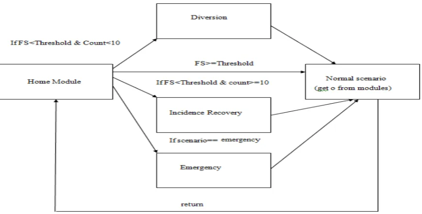
© 2015-19, IJARCS All Rights Reserved 44 Figure 2. Block Diagram for Proposed System
A. Home Module
The following algorithm shows the functioning of home module:
Home _function () { If (emergency) Diversion(); Else { 𝐹𝐹𝐹𝐹𝐹𝐹= 𝑄𝑄𝐷𝐷𝐹𝐹
𝑍𝑍𝑒𝑒𝑒𝑒𝑒𝑒
If 𝐹𝐹𝐹𝐹>𝑇𝑇𝑇𝑇 Normal(4); Else { (*p)=(*p)+1; If((*p)<=10) Incident_recovery() Else
Diversion(); }}
Higher priority is always assigned to emergency scenarios in which it is mandatory to divert the traffic on account of which always it is checked the existence of any such emergency. If the traffic is above a certain threshold it is perceived that normal scenario exists and normal conditions are present, otherwise either incident recovery or diversion tactics are followed based on the counter value. This is shown in Figure 2.
The functionality of the proposed system is divided into four modules:
• Main Module-normal scenario • Incident Recovery module
• Emergency module
• Low traffic module
B. Main Module (Normal Scenario)
This module is the basic model of the proposed system. The aim of this module is to determine green time by weighing in factors such as road conditions (quality),width
of the following lane, flow rate(speed) of the traffic ,traffic density, start-up time etc. this module. Any incident would have an impact on flow rate so a threshold value for flow rate is allocated which would determine the state of traffic.
1) Proposed algorithm
Normal scenario(int o){
//1 CYCLE TIME DETERMINATION { Decrement values above o by 1
SET ALL NECESSARY VALUES TO 0 For i=1 to o
If (𝑇𝑇𝑒𝑒𝑒𝑒𝑒𝑒)𝑛𝑛+1 (𝑇𝑇𝑒𝑒𝑒𝑒𝑒𝑒)𝑛𝑛 ≥ 0.8
(𝛼𝛼𝐷𝐷𝐹𝐹)𝑛𝑛= (𝛼𝛼𝐷𝐷𝐹𝐹)𝑛𝑛+ 1 For D=1 to o{ For r=1 to o
𝑊𝑊𝐷𝐷 = (∝𝐷𝐷𝐹𝐹∗ 𝑄𝑄𝐷𝐷𝐹𝐹) + 𝑊𝑊𝐷𝐷 // 𝑊𝑊𝐷𝐷 ,𝑊𝑊𝑇𝑇𝑇𝑇is made 0 before every iteration(cycle)
𝑊𝑊𝑇𝑇𝑇𝑇 =𝑊𝑊𝑇𝑇𝑇𝑇 +𝑊𝑊𝐷𝐷 }
Sort 𝑊𝑊𝐷𝐷 in descending order and assign i=1 to 4 in descending order
𝐶𝐶1=𝑊𝑊𝑇𝑇𝐶𝐶𝑇𝑇𝑇𝑇𝑇𝑇 for D=1 to o{
𝑍𝑍𝐷𝐷=𝑊𝑊𝑊𝑊𝑇𝑇𝑇𝑇𝐷𝐷 ∗c
𝑍𝑍𝐸𝐸𝐷𝐷 =𝑅𝑅1𝐹𝐹∗ 𝑍𝑍𝐷𝐷
𝑍𝑍𝑇𝑇𝑇𝑇 = 𝑍𝑍𝑇𝑇𝑇𝑇 + 𝑍𝑍𝐸𝐸𝐷𝐷
𝐶𝐶1= 𝐶𝐶1+𝑍𝑍𝑇𝑇𝑇𝑇 }
𝐶𝐶1=𝐶𝐶1 + 𝑇𝑇𝐹𝐹
//2.GREEN TIME DETERMINATION For i=1 to n
{ 𝑍𝑍𝑒𝑒𝑒𝑒𝑒𝑒 =𝑍𝑍𝐸𝐸𝐷𝐷+𝐹𝐹+𝐶𝐶𝐶𝐶𝑇𝑇
𝐶𝐶=𝐶𝐶 − 𝑇𝑇𝑒𝑒𝑒𝑒𝑒𝑒]𝑖𝑖 }}}
2) Determination of cycle time
Rabab Kazi et al, International Journal of Advanced Research in Computer Science, 7 (2), March- April, 2016,42-48
within 80 % of the higher lane, equal weightage is assigned to sectors 1 and 2. 𝛼𝛼𝐷𝐷𝐹𝐹 gives the weightage assigned to a particular sector while 𝑄𝑄𝐷𝐷𝐹𝐹 is the volume of cars in a distinct sector. The priority assigned to a particular direction in previous is given by i. 𝑊𝑊𝐷𝐷is the weightage for a direction which is 0 at beginning of every cycle.𝑊𝑊𝑇𝑇𝑇𝑇is the total weightage for all directions for a junction J.𝑇𝑇𝑇𝑇𝑇𝑇 is the total cars that passed through junction in previous cycle.
3) Determination of green time [2]
𝑍𝑍𝐷𝐷 is the ideal time which does not consider any factors. Road factor is obtained by weighing in factors such as quality of road and width of road. Traffic mainly moves in 3 directions so 3 road factors need to be accounted for. Directions 1, 2, 3 & 4 signify north, south, east and west respectively. One of the directions considered would flow for 2 phases due to lack of collisions, so the road factor considered would be maximum of the remaining 2 factors. 𝑍𝑍𝑅𝑅𝑇𝑇is the total time obtained by adding time added due to road factor (𝑍𝑍𝑇𝑇𝑇𝑇) with ideal time (𝑍𝑍𝐷𝐷) and 𝑍𝑍𝑒𝑒𝑒𝑒𝑒𝑒 is the effective time by considering road factors and start up time.
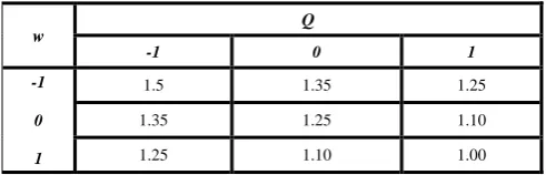
4) Road factor
Road factor is dependent mainly on 2 parameters: quality and width of the road. It is considered for outgoing lanes. The values of quality(Q) and width(W) are quantized to three levels - 0, 1, -1 wherein 0 signifies similar conditions and, 1 and -1 denote better and worse conditions than the current road, respectively. A road factor matrix is thus formed which is given as follows:
Table 1. Road factor
This is statically determined at the beginning of execution and can be updated by observing the collected data.
C. Incident Recovery Module
Whenever an incident occurs there is a direct impact on the speed of the traffic which is reflected by flow rate in the proposed algorithm. To deal with incidents, a threshold has been defined which determines a lower bound for the flow rate. Whenever the traffic is below that threshold, the system assumes that an incident has occurred and initiates a predefined function to divert the traffic from the affected lane. If no cars pass in the next cycle, then the traffic is dealt with the basic module, else it is assumed that the traffic is abnormally high on that lane and corresponding message is delivered to other junctions to regulate traffic and reduce flow in that direction. The algorithm can be defined as follows:
Incident recovery (D){ Normal scenario(D); return;}
Here D denotes the direction of traffic which is affected. The normal scenario then executes the traffic for the remaining scenarios.
D. Emergency Module
An emergency situation takes place when events such as fires and road accidents occur. During emergencies, vehicular traffic needs to be diverted from important routes to allow for the smooth transport of crucial vehicles. To do so it is necessary to divert traffic to other paths till the road has been cleared.
In such a scenario, all the junctions in the route are selected and marked as priority junctions. All the neighboring traffic junctions thus, reduce the traffic flowing to the concerned junction. In order to avoid congestion, the traffic junctions feeding traffic to these neighboring junctions also reduce the flow to the said junction. In such scenarios, the parameter 𝑍𝑍𝑒𝑒𝑒𝑒𝑒𝑒 is predetermined based on cycle duration time and the distance of the junction from the affected junction. A bottleneck situation may occur if the traffic is immediately diverted to the freed road. Thus, to avoid such situations, vehicles must be allowed to pass through in a controlled and regulated manner which will eventually stabilize the traffic flow.
E. Low Traffic Module
During the nights, the roads experience a lower traffic density as compared to those throughout the day. For this reason, in India, the entire traffic signal system is deactivated, leaving only pulsing yellow traffic lights on. Without any road regulations or restrictions to adhere to, people resort to negligent and irresponsible driving, due to which roads become perilous for drivers. This becomes apparent when multiple vehicles approaching a junction from different lanes collide on the road.
In this module, a signal that is green is allowed to remain green, as long as a car passes the stipulated threshold as shown in Figure 3. When a car crosses the threshold, if the remaining green time is less than 5 seconds, then 5 seconds are added to the clock timer. An upper and lower limit for the green time is defined so as to prevent a particular lane’s traffic signal from having a green signal for an excessive time period. The Low traffic Module allows for a range of green times, lying between 30 to 90 seconds so as to ensure optimal flow of traffic while minimizing wastage of fuel.
Figure 3. Flowchart for Low Traffic Module
IV. IMPLEMENTATION
In order to study the effects of the proposed algorithm, simulations were carried out using SUMO simulator along with MOVE software. SUMO is Simulation of Urban Mobility. It is a free and open source traffic simulation tool that can simulate real-world vehicular traffic flow. SUMO reads the input file and produces an output file by processing the simulation. Simulation of Urban Mobility (SUMO) along with MOVE software helps in simulating the necessary scenarios. SUMO simulator helps demonstrate the mobility of nodes, edges, etc from the MOVE software. SUMO was used to test the proposed algorithm on various urban infrastructures, the results of which were observed and optimized.
V. RESULTS AND DISCUSSIONS
The effects of growing congestion can not only be seen on the average speed of the traffic but also in the form of increased emissions and consumption of fuel. Thus, the evaluation of algorithms needs to be carried out not only on the basis of their impacts on speed but also on their impacts on the overall reduction of fuel consumption and emission. In the proposed system, the following scenarios were considered:
• Normal traffic conditions with varying density • Blocked Paths
• Low Traffic conditions
For every scenario, the results of the static and proposed algorithms were compared based on parameters such as speed, emissions and, fuel consumption.
A. Normal Traffic Conditions With Varying Density
1) Speed
Figure 4. Speed vs. Density - All cases
In Figure 4, the Normal scenario module is considered where no exceptional behaviour of traffic movement is observed such as undue blockages. From the graph it can be determined that with a gradual increase in traffic density, the speed of the traffic is reduced to a great extent when static times are used to handle traffic. Contrarily, when the proposed algorithm is used to manage traffic, the average speed of the traffic is reduced with increase in density, but the average speed of traffic is higher than observed speed given by static time determination.
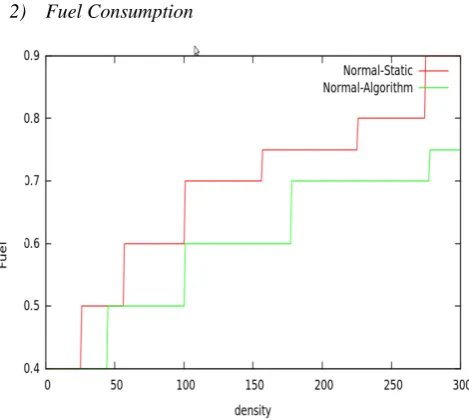
2) Fuel Consumption
Figure 5. Fuel vs. Density – Normal Scenario
Rabab Kazi et al, International Journal of Advanced Research in Computer Science, 7 (2), March- April, 2016,42-48
3) Emissions
Figure 6. Emission vs. Density - Normal Scenario
From Figure 6, it is seen that the impact of the proposed algorithm on emission is higher at lower densities of traffic as emission is considered for each vehicle and not for the entire traffic and at lower densities the speed of travel is higher, but with gradual increase in traffic the speed is reduced and within an optimum range. Emission is reduced not only for the proposed algorithm but also for static scenario, but on further increase in traffic a spike in emission is observed for static case while no such drastic increases are observed when the proposed algorithm is implemented. This is due to fact that speed is reduced below the optimum range at a much lower density of traffic for static case while speed only goes below the optimum range at much higher densities when proposed algorithm is implemented.
B. Blocked Path
1) Speed
In this scenario, a particular path was blocked off and vehicles were rerouted to other available lanes. Diversions contribute additional traffic load on other nodes. It was observed that the static algorithm was inefficient in such scenarios. The proposed algorithm handled such a scenario by efficiently varying time and thus reducing the impact on other junctions. In Figure 4, with a gradual increase in traffic density, the speed of the traffic is reduced to a great extent when static time is used to handle traffic. Contrarily when the proposed algorithm is used to manage traffic, the average speed of traffic is reduced with increase in density but the average speed of traffic is higher than observed speed given by static time determination.
2) Fuel Consumption
From Figure 7, it can be observed that at any particular density level the consumption of fuel is consistently lower for the proposed algorithm as compared to static case. The average fuel consumption in both cases is much lower as compared to other scenarios yet proposed algorithm gives better consumption rate by a miniscule margin.
Figure 7. Fuel vs. Density – Blocked Path Scenario
3) Emission
From Figure 8, it is seen that the impact of proposed algorithm on emission is higher at lower densities of traffic as emissions are considered for each vehicle and not for the entire traffic and, at lower densities the speed of travel is higher, but with gradual increase in traffic the speed is reduced and within an optimum range. Emissions are reduced not only for the proposed algorithm, but also for static scenario. With further increase in traffic, it is has been observed that there is a sharp incline in emissions for the static case, while no such spike is observed when the proposed algorithm is implemented. This is due to fact that speed is reduced below the optimum range at a much lower density of traffic for static case while speed only goes below the optimum range at much higher densities when the proposed algorithm is implemented.
C. Low Traffic Conditions
1) Speed
From Figure 4 given above, it can be observed that as traffic density increases, the speed of the traffic is reduced to a great extent when static times are used to handle traffic. However, when the proposed algorithm is used to manage traffic, the average speed of traffic is reduced with increase in density, but the average speed of traffic is higher than observed speed given by static time determination. Average speed is higher for proposed algorithm as compared to static with there being minute differences in the observed speed in both the scenarios despite the fact that the observable speed is moreover similar.
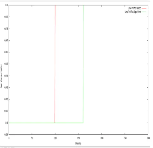
2) Fuel Consumption
From Figure 9, it is observed that the average fuel consumption in both cases is much lower as compared to other scenarios. However, the proposed algorithm gives a better consumption rate by a small margin.
Figure 9. Fuel vs. Density – Low Traffic Scenario
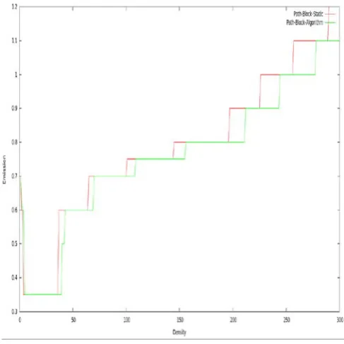
3) Emission
From Figure 10, it can be observed that the range of optimum densities for which emissions are minimal is much larger in both the cases, thus producing lower emissions. However, there are observable differences in their emissions, with the proposed algorithm showing better results. For example, with the proposed algorithm, for a density of 150 vehicles, emissions produced are approximately 0.34 units while for the static algorithm with the same density, emissions produced are approximately 0.35 units. These differences may seem to be insignificant, but the overall impact of implementing the proposed algorithm over larger regions is far greater.
Figure 10. Emission vs. Density – Low Traffic Scenario
VI. CONCLUSION
The purpose of this paper was to introduce a dynamic algorithm that focused on improving traffic conditions by enhancing the efficiency of traffic signals and junctions. The proposed algorithm was an improvement on existing algorithms in that it attempted to not only reduce traffic congestions but also, reduce fuel consumption and vehicle emissions. Our aim was to develop an algorithm that could dynamically manage traffic using parameters such as speed, density, fuel consumption and emissions. This included developing individual modules to handle different traffic scenarios such as, route diversion processes to handle incident and emergency scenarios. A start-up factor was introduced to aid in reducing the consumption and emissions. Another feature included using a time buffer between two phases to reduce collisions.
VII. REFERENCES
[1] Mario Collotta, Tullio Giuffre, Giovanni Pau,
Gianfranco Scata ,“Smart Traffic Light Junction Management Using Wireless Sensor Networks”,
WSEAS TRANSACTIONS ON COMMUNICATIONS, Volume 13, E-ISSN
2224-2864,2014.
[2] Farheena Shaikh, Dr. Prof. M. B. Chandak,“An
Approach towards Traffic Management System sing Density Calculation and Emergency Vehicle Alert“,IOSR Journal of Computer Science (IOSR-JCE) e-ISSN: 2278-0661, p-ISSN: 2278-8727,2014.
[3] T. Kalaivani, A. Allirani, P. Priya, “A survey on Zigbee based wireless sensor networks in agri- culture”, 3rd International Conference on Trendz in Information Sciences and Computing (TISC), pp. 85-89, 2011.
[4] Joseph Mathew, P. M. Xavier, “TRAFFIC
MANAGEMENT SYSTEMS”, IJRET: International Journal of Research in Engineering and Technology eISSN: 2319-1163,pISSN: 2321-7308,2013.
[5] Transport research wing of India, “ROAD
TRANSPORT YEARBOOK”, 2012.
[6] Andrew J Kean, Robert A Harley, Gary R Kendall,
“Effects of Vehicle Speed and Engine Load on Motor Vehicle Emissions”, Environmental Science and