Volume 3, No. 5, Sept-Oct 2012
International Journal Of Advanced Research In Computer Science
RESEARCH PAPER
Available Online At www.ijarcs.info
ISSN No. 0976-5697
Logistic regression and its implementation for email spam filtering
K.Srikanth*
Department of Computer Science SV University, Tirupati- 517 502
S. Ramakrishna
Professor, Department of Computer Science SV University, Tirupati- 517 502
K.V.S.Sarma
Professor, Department of Statistics SV University, Tirupati – 517 502
Abstract: This paper deals with an experiment on spam filters using Logistic Regression in which the efficiency of the filter is influenced by characteristics of the frequency distribution of the tokens. The focus of discussion lies on the need for data cleaning before developing the model. Features that are inconsistent shall be separated out before including them in the model. The UCI dataset showing the percentage of token counts in each mail is used in the model and the discriminating ability of the filter is studied with the help of ROC curve.
Keywords: spam, Roc curve, Logistic, UCI data.
I. INTRODUCTION
Logistic regression is a popular method used for binary classification. It is used as a filter to discriminate between spam mails and non-spam mails basing on the features of the e-mail. An unsolicited email is known as a spam mail. Though spam mails are not harmful, still some of them like phishing mails attract unwanted attention of the user. Several companies spend a significant amount of time on identifying and deleting spam mails.
There are different methods of filtering mails like white list- Black list method, content based filters, probability-based filters, statistical filters etc. The basic requirement in designing a filter is tokenization which means dividing the mail text into words, special characters and other important features. Each feature is called a token.
Classification of a mail into spam or non-spam is primarily based on the judgement of the user. The user may define a list of words or phrases and request to email provider to direct the receiving mail to the inbox or the junk box after comparing with the list. Those who send spam mails are often called spammers and they play a game with the user in sense that the user is mislead by the classification software. Words or addresses blocked by the users are slightly modified by the spammers so that spam mails escape the filter and enter the inbox.
It is therefore impossible to make an error free classification of mails in to spam or non-spam groups but basing on a training data one can define probabilistic rules which minimize the error of misclassification. This requires a large number (n) of mails which are classified as spam (n1)
or non-spam (n2), by a deterministic rule. This data is used
as a corpus.
The Naive Bayesian filter [1] is one simple and commonly used filter that is based on the posterior probability of a mail being spam (non-spam) given that it
giving importance to innocent tokens and using a prior distribution for spammy tokens. K.Srikanth, S.Ramakrishna and K.V.S Sarma [3] have combined Bayesian method using regression analysis to produce new filter.
II. PERFORMANCE MEASURES OF FILTERS
It is interesting to note that each token in a mail has some discriminatory power. For instance if the token ‘congratulations!!!!’ appears dominantly in spam mails and occasionally in non-spam mails, it is a good feature of a spam so that a mail having this word (with triple exclamation) can be marked as a spam. Similarly a sequence of capital letters (upper case) in the text is another feature and it will have its own power of classification. A commonly used measure of performance is % of misclassification calculated form the following table called confusion matrix by Kohavi and Provost [4].
Table-1: Confusion Matrix
Predicted Mail – type Actual Mail- type Spam Non-spam
Spam n11 n12
Non-spam n21 n22
The numbers in the matrix represent the count of mails in each pair of classes. n11 and n22 are correctly classified
mails while others are misclassified mails. Associated with each feature, we can define a measure denoted by X. Then there exists a cut-off (c) such that a mail is classified as spam if X > c. Thus the confusion matrix depends on the feature X and cut-off (c). In general there could be k features X1,X2,...,Xk with corresponding cut-off values
c1,c2,....,ck.
Precision and Recall. More details in this area can be found in Margaret Dunham and S.Sridhar [5] and Han and Kamber [6].
III. REGRESSION BASED FILTERS
Statistical regression is a method of summarising information from several explanatory variables into a new score (Y) which is a weighted function of the tokens. When a linear model is used, the score takes the form β0+ β1 X1+
β2X2+...+ βkXk where βi is the coefficient of Xi (i =
1,2,...,k) to be estimated from the data and β0 is a constant.
In the general linear regression model Y will is assumed to be a continuous random variable following normal distribution. The weights are then estimated by a method called Ordinary Least Squares (OLS) method. But in the classification of mails, Y is binary variable taking values 0 (non-spam) and 1(spam) and the weights cannot be estimated using OLS method.
In the classification problem we are interested in estimated P[Yi= 1] to mean the probability that ith case is a
Spam. This is done by using a Logistic Regression (LR) model given by
(1)
and P[Yi = 0] = 1 – P(Yi = 1].
More conveniently we can see that =
. This quantity is called the logit.
We are ultimately estimating the probability that a mail is spam given that it has values Xi as given in the mail and
betas are the weights estimated from training data.
Once the model coefficients are estimated the model is ready for testing on already known cases so as to evaluate the performance of the classifier.
In the present case the variable Xi refers to a measure on
a token of the text. This can be a continuous variable, like the proportion of times the token appeared in the text. It can also a categorical variable taking values 0 (taken absent in the text) and 1 (token present in the text). Using any statistical software like SPSS we can fit the LR model to the testing data and estimate P(Yi = 1]. Assuming that that a
mail is equally likely to be a spam or non-spam, we take the
cut-off as c = 0.50 and the decision rule is as follows. "If P(Yi = 1] > 0.50 classify the mail as spam; else as
non-spam"
For each mail in the test data we implement this model calculate score which is converted into probability. It is called predicted score from which predicted class membership can be found.
The cross tabulation of actual and predicted scores gives the confusion matrix from which we find the percentage of misclassification.
In the following section we visit a dataset from UCI repository to build the LR model taking the entire data as training set. We implement this model on Enron Data set (another repository) and study the efficiency of the LR model.
IV. THE UCI DATA SET AND THE ENRON DATA SET
The UCI data set was created by George Forman, Erik Reeber, George Forman and Jaap Suermondt [7]. It is a processed data, available with several tokens and features as columns. Out of 4601 mails of the set 1813 were Spam (39.4%) while 2788 (60.6%) were non-spam. The data set contains 54 continuous variables taking values between 0 and 100 out of which 6 variables are special characters
and the others are words. They represent the percentage of cases containing the given word in the mail. It is obtained as 100 (nw/N) where nw = number of time the word w
appears in the given mail and N is the total number of words in the mail. The total run-length of capital letters (upper case) is also measured for each mail and treated as a feature that can be correlated to the class of mails. The average
and the longest capital run length are also measured and recorded for each mail.
The Enron data set [8] is another repository of mails that were classified as spam and non-spam. It contains 1324 mails with 322 spam and 1002 non-spam mails. The content of each mail from data set will be used to tokenize the message and apply the LR model for classification on this data set as testing data set.
V. STATISTICAL FEATURES OF THE DATASET
The data shows very inconsistent values for each token as evidenced by the descriptive statistics of selected tokens given in table-2.
We observe the following from table-2.
a. The incidence of each token has a large spread around the average as can be seen from the standard deviation and the coefficient of variation.
b. The distribution of many tokens is positively skewed in both spam and hams sets (Figure-1)
c. The capital_run length letters is highly skewed to right indicating that longer run lengths have shorter chance of occurrence (Figure-2)
Table-2: Descriptive statistics for selected tokens
Token/ Feature Mail Type Mean Std. Deviation Skewness CV
“make” Spam 0.152339 0.310645 3.973379 203.9173
Non-Spam 0.073479 0.297838 7.139184 405.3371
“our” Spam 0.263245 0.703950 4.885845 267.4123
Non-Spam 0.100789 0.567850 8.754640 563.4042
“over” Spam 0.174876 0.321927 2.559845 184.0889
Non-Spam 0.044544 0.222888 12.45525 500.3707
“$” Spam 0.174478 0.360479 8.038261 206.6038
Non-Spam 0.011648 0.069647 14.24015 597.9035
capital_run_length_total Spam 470.6194 825.0812 7.415522 175.3181 Non-Spam 161.4709 355.7384 6.521542 220.3111
Figure-1: Distribution of the percentage incidence of the token over
Figure-2: Distribution of the capital_run length
Remove records having length beyond a certain value.
VI. THE LR MODEL AND PREDICTION
The training data for developing the model is the complete set of 4601 records of UCI data set [7] and the model is developed using SPSS.
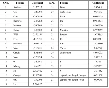
All the 59 variables (features) are included in the model with mail_type as the dependent variable. Stepwise forward conditional method is issued for the selection of variables into the model. At the 35th step the LR algorithm got terminated. Out of 59 variables (predictors) only 35 got selected into the model with the weights (regression coefficients) shown in table-3 along with a constant 1.492992 for the model.
Two important characteristics i) Predicted Probability (of spam) and ii) Predicted Group Membership are are of interest for each mail. Each mail in the testing data is evaluated with this model and the resulting probability P[Y = 1] is stored. Whenever P[Y = 1] > 0.5 the mail is classified as spam.
The performance of the LR model is studied in terms of i) % of correct classification and ii) ROC curve. SPSS automatically produces a classification table at the end of the 35th step which shows 92.41% of mails correctly classified. In terms of confusion matrix given in section-2, we get n11 = 1597, n12 = 215, n21 = 134 and n22 = 2654. The model has correctly classified 1597 spam mails and 2654 non spam mails. The False Positive Rate is 2.9% (134 out of 4601) and False Negative rate is 4.67% (215 out of 4601) and total misclassification rate of the model is 7.59%. The ROC curve shown in figure-3 has an Area Under Curve (AUC) = 0.9759. It means that when tested with the LR model a randomly selected mail from the testing data having the list features of table-3, is 97.59% more likely to be spam than a non spam.
In the following section we develop a procedure to test this model with a different data set, the Enron data [8].
VII. VERIFICATION AND TESTING
The Enron data set has 1305 mails already classified as spam and non-spam. We apply the LR model on this data set and estimate the classification accuracy.
Algorithm-1
a. Set R = {X1, X2,....,Xp} as the array of tokens in the
LR model.
b. Set B = {b0, b1,b2,...,bp} as the array of coefficients
in the LR model
c. Set W = {w1,w2,...,wn} as the array of tokens
obtained from the ith message n (< = >) p d. For the kth message, set score(k) = b0
e. If Xi∈W then score(k) = score(k) + bi
f. Find = exp(-score(k))
g. If > 0.5 classify the kth mail as Spam
else non-spam
h. Repeat until all the mails are classified.
In order to test the data on the Enron data set, we have designed a new scheme of random testing by picking up a desired number of mails at random from the data set. The interesting thing is that a random subset of mails may contain an arbitrary number of spam or non-spam mails. By repeatedly testing the model on random sets, the model efficiency can be evaluated. Consider the following algorithm
Algorithm-2
a. Select the desired sample size n
b. Pick up a random sample of n mails from the list c. Classify each mail using algorithm-1
d. Find the misclassification rate(percent) π
e. Repeat with different sample sizes and compare π
f. Calculate the average π and its summary statistics. The experimental set up was done using MS-Access database and a VB code given in the appendix.
VIII. OBSERVATIONS
The statistics of classification obtained from the experiment are shown in table-4.
The False Positive Rate (FPR) is 5.78 ± 0.202 and the False Negative Rate (FNR) is 2.50 ± 0.487, where the values represent mean ± standard error. The LR model therefore has lower FNR than FPR but the FPR is more consistent than the FNR due to lower standard error.
When a random sample of messages of size n is selected from the main list they are stored in another table and a code is written to produce only distinct messages as sample (avoiding redundancy). In order to assess the effect of sample size on the classification process, each trial is repeated four times with the corresponding sample size and the misclassification rate is recorded.
Figure-4 shows the percentage misclassification which has an average of 9.369 with 95% confidence interval (9.266, 9.472). The trend is also stable as the sample size increases.
Table-3: Predictors and coefficients
S.No. Feature Coefficient S.No. Feature Coefficient
1 Address 0.122712 19 Data 0.82611
2 Our -0.28388 20 technology -0.96693
3 Over -0.83499 21 Parts 0.662809
4 Remove -2.48762 22 Pm 0.959694
5 Internet -0.60396 23 Cs 40.00309
6 Order -0.58385 24 Meeting 2.773859
7 Will 0.175134 25 Project 1.675863
8 Free -1.15031 26 Re 0.830611
9 business -1.08472 27 Edu 1.524589
10 You -0.10451 28 Table 2.94731
11 Credit -1.51498 29 conference 4.069203
12 Your -0.20924 30 ; 0.91216
13 0 -2.20861 31 ! -0.356
14 Money -0.4823 32 $ -5.29363
15 Hp 2.593462 33 # -3.07652
16 George 11.93764 34 capital_run_length_longest -0.01108
17 650 -0.32904 35 capital_run_length_total -0.00079
Figure-3: ROC curve: AUC = 0.9759
Table-4: Classification Statistics with Different samples sizes (figures in the bracket indicate % of cases)
Trial Sample size True Positive cases True Negative cases False Positive cases False Negative cases % misclassification (π)
1 20 13 (65.00) 06 (30.00) 1 (5.00) 0 (0.00) 5.00
2 50 44(88.00) 02(4.00) 3(6.00) 0(0.00) 6.10
3 100 81(81.00) 10(10.00) 7(7.00) 1(1.00) 8.08
4 200 161(80.00) 23(11.50) 10(5.00) 6(3.00) 8.00
5 350 267(76.29) 51(14.57) 18(5.14) 14(4.00) 9.10
6 500 384(76.80) 69(13.80) 29(5.80) 17(3.40) 9.20
7 600 462(77.00) 82(13.67) 36(6.00) 19(3.17) 9.10
8 750 581(77.47) 100(13.33) 41(5.47) 27(3.60) 9.00
9 900 697(77.44) 117(13.00) 55(6.11) 30(3.33) 9.40
10 1000 766(76.60) 135(13.50) 63(6.30) 35(3.50) 9.81
Figure-4 % Misclassification in Repeated samples of different sizes
IX. DISCUSSION
Implementation of LR model is based on tokenization of the message. It is possible that a message may not have single token that matches with the variables of the LR model. In that case the score becomes constant = 1.492992 and P[Y =1] = 0.18349 and the message is classified as non-spam. This LR model is however static in the sense that the coefficients are estimated by the training data from the UCI data set. To make the model dynamic one needs to include new tokens, in which case the LR model has to be evaluated
matches with the model tokens, we get score = 0 and P[Y =1] = 0.5 and the messages is classified as non-spam!
X. REFERENCES
[1] M. Sahami, S. Dumais, D. Heckerman, E. Horvitz "A Bayesian approach to filtering junk e-mail". AAAI'98 Workshop on Learning for Text Categorization 1998.
[2] Paul Graham, “A plan for spam”, 2002.
www.paulgraham.com/spam.html.
[3] K.Srikanth, S. Ramakrishna and K.V.S.Sarma, “An
Information Technology and Knowledge Management, January-June 2012, Vol. 5, No. 1. pp-169-175.
[4] Kohavi and Provast, “Glossary of Terms”, Machine
Learning, 30, 271-274 1998
[5] Margaret Dunham and S.Sridhar, “Data Mining
Introductory and Advanced Topic” 2006
[6] Jiawei Han and Micheline Kamber, “Data Mining
Concepts and Techniques” 2005
[7] UCI Data repository by George Forman, Erik Reeber,
George Forman, Jaap Suermondt from the mails collected during June-July 1999.
[8] Enron Email Dataset prepared by CALO project 2004
Appendix: Portion of code for evaluating the LR model Private Sub evaluate()
rs2.Open "select * from temp ", db1, adOpenStatic, adLockOptimistic
Do While Not rs2.EOF t1 = rs2!content
'Calculation of Capital_run length Dim uc As Integer IsNumeric(ww) = False Then uc = uc + 1
Print "Score = "; Format(score, "0.00000") If score <= 0.5 Then
rs2!new_type = "0"
Print "Predicted class = ", "Non-Spam", score Else
rs2!new_type = "1"
Print "Predicted class = ", "Spam", score End If