International Journal of Advanced Research in Computer Science RESEARCH PAPER
Available Online at www.ijarcs.info
© 2010, IJARCS All Rights Reserved 7
Design and Analysis of a Reverse Hierarchical Graph Search Algorithm
Lopamudra Nayak*
Graduate Student, Department of Computer Science Jackson State University
Jackson, MS, USA [email protected]
Natarajan Meghanathan
Associate Professor, Department of Computer Science Jackson State University
Jackson, MS, USA [email protected]
Abstract: During the process of searching for an element in Directed Acyclic graphs (DAGs), traditional search algorithms like Depth First Search (DFS) waste lot of time in backtracking. This paper presents an alternate search algorithm, known as the Reverse Hierarchical Search (RHS) algorithm, for DAG/tree data structures. The RHS algorithm promises better performance over the DFS algorithm by avoiding path retracing. This research puts focus on DAG/tree-like data structures with lineage elements. Based on the purpose the data structure solves, hierarchical tree structures have related elements that are organized in a certain way. The knowledge of the purpose of the data structure helps in creating a basic criterion for locating and adding new members. The RHS tree is based on searching for an element in a reverse hierarchical order. All nodes that are found in the search path are added to the solution space. To avoid crowding the solution space with revisited nodes, any previously visited node information is re-used and duplicity of nodes is prevented. This makes the RHS algorithm to be more scalable than DFS. In terms of run-time complexity, RHS is a better performer than the DFS algorithm for linear tree/ DAG data structures.
Keywords: Hierarchical Search, Recursion, Directed Acyclic Graphs, Trees, Lineage Elements
I. INTRODUCTION
In the field of computer science, a data structure is a particular way of storing and organizing data in a computer so that it can be used efficiently. Data structures are considered to be very critical for the efficiency of many algorithms as well as to manage huge amounts of data, including large databases and Internet indexing services. Both data structures and algorithms form the key components in software design and to develop highly efficient and effective software [1]. It is critical to choose the best algorithm and data structure for a particular task. Selection of an unfit algorithm to start with, plausibly may fail to produce optimal results irrespective of the number of micro-level adjustments or patches that may be applied at later stages. Selecting an algorithm usually involves a careful analysis of the associated tradeoffs. While a particular algorithm might be the best solution for a certain type of data, it may perform notably sluggish as the dataset changes. For instance, there is no single sorting algorithm that can be identified as the most advantageous in all scenarios. The deciding factor is the way the algorithm would be used and the best approach lies in choosing the solution that provides the best results most of the time, if not always.
Different kinds of data structures are suited to different kinds of applications, and some are highly specialized to specific tasks. Data structures may be grouped into three categories, based on the level of complexity as Primitive, Composite and Abstract.
(a) Primitive data structures are defined as a data type for which the programming language provides built-in support. Examples of Primitive data structures in programming languages include boolean, char, double and float.
(b) Composite datatypes may be heterogeneous combination of primitive data structures. For example, the struct construct in C++ given below,
models an Account object holding dissimilar data structures like integer, character and float.
struct Account { int account_number; char *first_name; char *last_name; float balance; };
(c) Abstract datatypes are solely theoretical entities, used to abridge the illustration of abstract algorithms, to order and appraise data structures, and to properly describe the type systems of programming languages. Examples of abstract datatypes are stack, tree, and queue.
There are two broad categories of data structures when classified based on their linearity: linear data structures and non-linear data structures. In a linear data structure, every item is related or attached to the previous and next item in a linear order (e.g. Arrays). In a non-linear data structure every element or member is connected to multiple elements in certain ways to mirror specific relationships (e.g. n-ary tree) which puts the data items out of sequence [2].
systematizing data objects based on keys as well. Several areas where trees are put to practical use are narrated below.
(a) Trees can hold objects that are sorted by their keys [4]. The nodes are ordered such that all keys in the left sub-tree of a node are lower in value than the current node, and all keys in the right sub-tree are larger than the current node’s key.
(b) Trees can hold objects that are strictly ordered by categories and located by sequences such as library books. Modeling a library of books can be done using a tree data structure since it can contain objects located by keys in sequences.
(c) Trees find use in language processing programs to represent phrase structure of sentences while constructing a parsing tree [2]. For example, during the process of compiling a Java program, the Java compiler first checks the grammatical structure of the source code and tries to build the parsing tree. Upon successful completion, this parsing tree guides the Java compiler to produce the executable.
(d) One instance of tree data structure, the B-tree, is particularly well-suited for implementation of databases. The challenge in database implementation is search time overhead caused due to disk read delays and inconsistencies caused by insertion or deletion [4]. The B-tree maintains a sorted order of records that enables sequential traversal. The number of disk reads is minimized by using a hierarchical index. Insertions and deletions are faster in a B-tree due to use of partially full blocks. Further, a B-tree minimizes the non-use of the interior nodes by ensuring optimal usage. Apart from databases, B-Trees are also used in file systems to provide random access to a particular section in the file.
The rest of the paper is organized as follows: Section 2 establishes the foundation by delving into several well-known search algorithms and their performance analysis; thereby, identifying any scope of improvement and choosing a suitable tree model to aid in the implementation of the proposed Reverse Hierarchical Search (RHS) algorithm. Section 3 explains the RHS algorithm, its algorithmic complexity and discusses the data model. Section 4 concludes the paper.
II. LITERATURE REVIEW OF TREE SEARCH
ALGORITHMS AND THEIR ANALYSIS
This section presents a review of the related work available in the literature on search algorithms in the domain of tree data structures and investigates any scope for improvement.
A. The Depth First Search Algorithm
Depth First Search (DFS) is a tree or graph traversal algorithm optimized for faster searching [6]. The search typically commences at the root of the tree and continues to explore each branch till the leaf nodes, before backtracking. As soon as the search reaches the leaf node/dead end, the control returns to the most recent node that has not been explored. DFS is closely related to preorder traversal of a tree. A preorder traversal simply visits each node before its children. In order to convert the preorder traversal into a graph traversal algorithm, the “child” node is replaced by “neighbor” node. Further, in order to optimize the algorithm
and prevent infinite loops, one would restrict the number of visits to each vertex. In order to enforce this restriction, marks are used to keep track of the visited vertices. This search may be used to build a spanning tree with certain useful properties.
The Depth First Search (DFS) algorithm begins with initializing a set of markers in order to identify the pre-visited vertices. Upon choosing a starting vertex ‘x’, a tree T is initialized to x, and Depth First Search(x) algorithm is invoked. The order of traversal of the vertices beginning from a vertex having multiple neighbors makes little difference. The graph shown in Figure 1 illustrates the application of the DFS algorithm.
Figure1. Graph Used for Applying DFS
Assuming the left edges in the graph are picked prior to the right edges while performing a DFS, commencing at vertex ‘A’, for a search that presumably memorizes pre-visited nodes (in order not to repeat them), the nodes will be ordered as A, B, D, F, E, C and G. The result of this search is a structure known as the Trémaux tree. Performing the same search without any knowledge of pre-visited nodes accounts for a different order of nodes : A, B, D, F, E, A, B, D, F, E etc. with infinite loops caught in the A, B, D, F, E cycle and inability to reach nodes C or G.
speaking, the run-time complexity is evaluated as O(bd
B. Iterative Deepening Depth First Search Algorithm
) with branching factor b anddepth d.
Applying the DFS to traditional search problems in the field of Artificial Intelligence happens to be a potential stress test. The exceptionally large size of the graph results in non-termination issues that are based on the infinite path length in the search tree. This seems to be an inherent lacuna in the algorithm. Besides, due to the limitation in the availability of memory, applying a data structure that records all pre-visited vertices will impose practical hindrance. In this scenario, the search time remains linear in the number of extended vertices and edges (may not be same as the size of the entire graph as some vertices might have been searched multiple times, while others may not at all be). In a situation where the depth limit is not known beforehand, a variation of the DFS algorithm may be applied to overcome the problem of infinite looping and in-accessible nodes, known as the Iterative deepening Depth First Search (IDDFS) [5]. The core idea is to run a depth-limited search over and over again, with each successive iteration incrementing the depth limit until one arrives at the depth of the shallowest goal state. IDDFS is viewed as a hybrid between Depth First Search and Breadth First Search, respectively inheriting the space-efficiency as well as completeness attributes. It is a preferred choice when the path cost is a non-decreasing function of the depth of the node.
Assuming ‘b’ as the branching factor and ‘d’ as the depth of the most superficial goal, the space complexity of the IDDFS algorithm is defined by O(b*d). The time complexity of IDDFS in well-balanced trees is same as Depth First Search i.e. O(bd
d d d
b b b b
d db
d+ + + − + + + +
= 2 (−2) ( −1)
[image:3.595.358.513.353.471.2]2 3 ... )
1 ( ) 1 (
). As is observed, iterative deepening search indulges in visiting states multiple times, the nodes on the lowest level are expanded once, those located in the penultimate layer to bottom level are expanded twice, and so on so forth. Gradually gravitating towards the root of the search tree yields an expansion of d + 1 times [5]. Computation of the total number of expansions in an iterative deepening search results in the following formulae:
∑
= + −d i
i b i d
0( 1 )
Assuming a scenario where b = 10 and d = 5, the total number of expansions is calculated as: 6 + 50 + 400 + 3000 + 20000 + 100000 = 123,456.
To summarize, an iteratively deepening search beginning from depth value of one through d enlarges about 11% more nodes than a traditional breadth-first or depth-limited search to depth d, while b is equal to ten. It is observed that higher the branching factor, the lower the overhead of repeatedly expanded states, but even when the branching factor is 2, iterative deepening search only takes about twice as long as a complete breadth-first search. This means that the time
complexity of iterative deepening is still
O
(
b
d)
, and the space complexity is O(b*d). IDDFS has an upper hand in space complexity while the time complexity suffers badly as depth of the tree increases. It is a preferred option for games where the requirement is to find shortest paths to a problem. However, the algorithm faces major bottleneck when it has to solve trees involving long search paths. As the value ofdepth (d) increases, the cost involved in terms of time increases multiple folds [6].
C. Scope for Improvement
As observed in the previous sections, popular tree search algorithms (including DFS and IDDFS) use heuristic-based tree pruning techniques like “backtracking” that consume a significant amount of search time at the expense of efficiency [5]. Backtracking is defined as a general method for exploring all (or some) solutions to a computational problem that incrementally builds nominees to the solutions. Each partial nominee n is discarded ("backtracks") as soon as it is determined that n possibly cannot be completed to reach a valid solution [5].
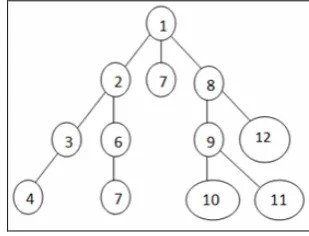
The DFS algorithm is based on vertical search path that explores available sub-trees; traversing and re-traversing (manifested as backtracking) the nodes until the target node is found. As depicted in Figure 2, a search for the target node requires navigation through at least thirteen nodes of which three are re-traversed. In Figure 2, node 1 represents the root node while 2 through 12 are the intermediate nodes. Node 10 represents the target node. The total time spent in reaching the target node calculated using equation 1, given that the depth of the tree is 3 and branching factor is 2 is computed as: 4 + 3*2 + 2*4 = 18 time units.
Figure 2. Schematic Representation of a Depth First Search Tree
From manual inspection, it can be identified that the successful path traversals leading to the target node is a straight path from the root as shown in Figure 3. A comparison of both these scenarios yields a performance ratio of 0.22 (computed as a ratio of time units used without backtracking to time units used with backtracking) explaining the penalty that the DFS algorithm pays for relying on backtracking.
Figure 3. Path of Successful Tree Traversal without Backtracking
III. DESIGN AND ANALYSIS OF THE REVERSE
HIERARCHICAL SEARCH (RHS)ALGORITHM
A. General Idea
The contribution of this paper is the design and development of a tree search algorithm hereafter referred to as Reverse Hierarchical Search (RHS) algorithm. The proposed optimization will provide a novel graph traversal algorithm for better time and space complexity as well as completeness for tree data structures. The proposed RHS algorithm is an uninformed [5] search similar to the normal DFS. However, unlike the DFS algorithm, which travels downstream from the root to leaf nodes, the RHS algorithm keeps a tab on backtracking by limiting the depth of search from individual nodes to the root. This enforced restriction of the search space boundary (i.e. upstream node till root) prevents indefinitely deep paths during traversals. The DFS algorithm begins the search vertically downwards in pursuit of the target node. Until the search element is reached, the algorithm backtracks (self repetitions without further advancement) to the penultimate junction nodes. For a complete binary tree of depth n, the worst-case search time complexity would be O(2n -1). Usually, in tree structures the root is a single element node while the maximum number of elements occurs at the nth level. Therefore, a search commencing at the level “n” would represent a logical initiative in reducing the volume of search by 2(n-1) elements (accounting for members at the nth
B. Selection of a Suitable Tree Model
level). Nevertheless, the proposed novel search algorithm is not
limited to binary trees and can very well be adapted for non-binary versions. Since the search terminates at the root, no backtracking will be necessary and all the child-parent nodes following a reverse hierarchy are added up to the solution space. This saves the users from revisiting the same path for further target searches. It is noteworthy that every single node that is traversed once gets into the domain of the solution space. In this approach, special emphasis will be given for optimization of the algorithm for tree structures with lineage elements.
[image:4.595.39.281.611.753.2]The studies will be based on a search model currently in use for student enrollment in most academic programs. Before registering for an advanced course a student has to establish his/her proficiency in the basic course curriculum referred to as “pre-requisites”. At the present time, some universities including Jackson State University (JSU) employ a manual transcript analyses that ensures that the student has satisfactory performance in previous classes on a case-by-case basis.
Figure 4. Pre-requisite Tree for Undergraduate Courses in Jackson State University CSC Department
Designing the RHS algorithm for the checking the pre-requisites will serve a three-fold purpose such as: (i) Assessment of validity/utility of the proposed modified DFS algorithm, (ii) Precise determination of student’s eligibility, and (iii) Efficient and economic usage of university’s resources by substituting the manual practice with an automated process.
C. Study of the Data Model
The pre-requisite tree (depicted in Figure 4) when observed closely is a directly acyclic graph (DAG) due to child nodes being shared among parents. The pre-requisite DAG is used to access information about the enrollment requirements for the courses. This DAG is a connected network of nodes (represented by individual courses) related to each other with a parent-child connection.
The left-most node is the root with the arrow pointing toward its children. The concept of one course having multiple pre-requisites is well modeled in the DAG. For optimization purposes, the courses have been segregated into four different years of undergraduate study (viz., freshman, sophomore, junior and senior). Each node in the tree is labeled with the code for the classes.
D. Informal Description of RHS
An informal description of the RHS algorithm is presented here:
1. Establish the vertex where the search should commence and assign the maximum search depth
2. Verify if the current vertex is the Goal State
• If no: Go to Step 3
• If yes: return
3. Verify if the current vertex is within the maximum search depth
• If no: Do nothing
• If yes:
Expand the vertex and save all of its predecessors in a stack
Call RHS recursively for all vertices of the stack and go back to Step 2
E. Formal Description of RHS
A Goal State is the final state after which traversal stops. A vertex having no un-traversed edges is said to be in Goal state.
The formal pseudo code for the proposed algorithm is presented here, which will be subjected to preliminary testing and search time complexity computation.
RHS (node, goal, depth) {
if (node = goal) return node; push_stack(node);
while (stack is not empty) { ……….Step (1) stack_counter ++;
If (depth > 0) {
nodeList_recvd := expand (node) While( nodeList_recvd is not empty ) { node = nodeList_recvd [next node] RHS (node, goal, depth-1) … Step (2)
Else
// no operation }
}
Expand (node) .……… Step (3) { i = 0
while ( node is not root ) { i++
if ( depth > 0 ) { For each edge e {
nodeList[i] := node.Parent(); // Fetch all parents of current node }
} }
Return nodeList; }
F. Asymptotic Complexity of RHS Algorithm
The computation of the run-time complexity of an algorithm is an important aspect for performance evaluation. The estimation of the run-time complexity of the RHS algorithm is narrated in this section. With reference to the steps narrated in the formal description of the algorithm in the previous section, for an input of size N (equivalent to the number of pre-requisite courses that exist for the desired course), step 1 is executed log (N) times. Similar to step 1, step 2 is executed log (N) times and so is step 3. Therefore, the total number of iterations needed to compute the RHS algorithm is: log (N) * log (N) + log (N) = log (N2
)
1
(
b
−
) + log (N) = log (N), ignoring the first term in the expression, which becomes negligible as size of N increases. A logarithmic run-time complexity for the RHS is considerably well lower than the linear run-time complexity for popular algorithms like the DFS.Evaluation of space complexity of the algorithm presents an estimate of the memory requirement for running the algorithm. With memory devices becoming cheaper day by day, space complexity results can bear moderately lower performance. During tree traversal, the memory needed in the original DFS is high when one reaches to the root of the tree. A branching factor ‘b’ for each node refers to average number of branches at any level. When a tree with depth d is inspected, the total number of nodes/vertices collected in memory is a combination of the expanded nodes up to depth ‘d’ and the current node being studied. There being
number of expanded nodes at each level, the total amount of memory that is required is computed as
2
/
)
1
(
*
*
)
1
(
)
1
)...
2
(
)
1
(
(
*
)
1
(
1
.
)...
1
(
*
)
1
(
)
1
(
*
+
−
=
−
+
−
+
−
=
−
−
+
−
d
d
b
d
d
d
b
b
d
b
d
=
b
*
d
2 (ignoring constant terms) = O(bd)G. Algorithm Application
Based on the requirements during student registration, a couple of scenarios have been isolated to evaluate the performance of the algorithm in a node-based model (see Figures 5 and 6).
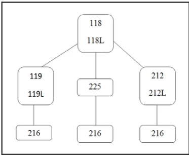
Scenario 1: Transcript analysis for registration of a single course (i.e. CSC216) depicted on a node based model is
[image:5.595.343.530.101.254.2]shown in Figure 8. Computing the processing time for this scenario gives the following results: Log2 (N) = log2 (7) = 2.80735 time units
Figure 5. Transcript Analysis for a Single Course in Node Based Model
[image:5.595.335.539.347.538.2]Scenario 2: Simultaneous transcript analysis for two courses (i.e. CSC216 and CSC450) yields a dataset of size N (N=10). Plugging the values of this scenario in the time-complexity equation derived in the previous section yields a computation time of 3.321time units (Log2(10)).
Figure 6. Transcript Analysis for Two Courses in Node Based Model
IV. CONCLUSIONS
Every element in the tree is indexed and positioned in a specific place in RHS algorithm. While in the DFS algorithm elements are thrown into the tree in a random fashion, the RHS algorithm relies on re-structuring the tree for optimization purposes. Every graph has a certain purpose and based on that the rearrangement is done. Once the criterion of re-structuring is set, every new element that comes in has a specific destination. The proposed RHS algorithm is based on a search process that begins its search from the leaf element at the nth level of the tree and not the root. In lineage tree structures, the nodes at subsequent levels are related to each other through parent child relationships. The parent elements found along the search path from the nth
V. ACKNOWLEDGMENTS
level to the root are added to the solution space following reverse hierarchy. Any other searches that follow a common path reuse the information in the solution space, improving the overall efficiency of the algorithm. The RHS algorithm is evaluated to have an asymptotic run time complexity of O(log (N)) and space complexity of O(N) for an N-node graph. Thus, the RHS algorithm is a valuable addition to search for ancestor-descendant relationships [7] in trees and directed-acyclic graphs.
This research is partly funded through the U. S. National Science Foundation (NSF) grants EPS-0556308 on Modeling and Simulation of Complex Systems and DUE-0941959 on Incorporating Systems Security and Software Security in Senior Projects. The views and conclusions in this document are those of the authors and should not be interpreted as necessarily representing the official policies, either expressed or implied, of the funding agency.
VI. RFERENCES
[1] T. H. Cormen, C. E. Leiserson, R. L. Rivest and C. Stein, Introduction to Algorithms, 3rd
[2] A. W. Appel and J. Palsberg, Modern Compiler Implementation in Java, Cambridge, MA: MIT Press, 1998.
Edition, Cambridge, MA: MIT Press, September 2009.
[3] N. Gelfand, M. T. Goodrich and R. Tammasia, “Teaching Data Structure Design Patterns,” Proceedings of the 29th
[4] R. Bayer, “Binary B-Trees for Virtual Memory,” Proceedings of ACM SIGFIDET Workshop on Data Description, Access and Control, pp. 219-235, San Diego, CA, USA, 1971.
SIGCSE Technical Symposium on Computer Science Education, vol. 30 (pp. 331-335), Providence, RI, USA, 1998.
[5] A. Reinefeld and T. A. Marsland, “Enhanced Iterative Deepening Search,” IEEE Transactions on Pattern Analysis and Machine Intelligence, vol. 7, no. 16, pp. 701-710, 1994.
[6] R. Tarjan, “Depth First Search and Linear Graph Algorithms,” Proceedings of the 12th
[7] S. Baskiyar and N. Meghanathan, “Binary Codes for Fast Determination of Ancestor-Descendant Relationship in Trees and Directed A-cyclic Graphs,” International Journal of Computers and Applications, vol. 10, no. 1, pp. 67-71, March 2003.