Exploiting Semantic Information for HPSG Parse Selection

Exploiting Semantic Information for HPSG Parse Selection

Sanae Fujita,♥Francis Bond,♠ Stephan Oepen,♣ Takaaki Tanaka♥

♥_{{sanae,takaaki}@cslab.kecl.ntt.co.jp,} ♠ _{[email protected],} ♣_{[email protected]}

♥_{NTT Communication Science Laboratories, Nippon Telegraph and Telephone Corporation}

♠ _{National Institute of Information and Communications Technology (Japan)}

♣_{University of Oslo, Department of Informatics (Norway)}

Abstract

In this paper we present a framework for experimentation on parse selection using syntactic and semantic features. Results are given for syntactic features, depen-dency relations and the use of semantic classes.

1 Introduction

In this paper we investigate the use of semantic in-formation in parse selection.

Recently, significant improvements have been made in combining symbolic and statistical ap-proaches to various natural language processing tasks. In parsing, for example, symbolic grammars are combined with stochastic models (Oepen et al., 2004; Malouf and van Noord, 2004). Much of the gain in statistical parsing using lexicalized models comes from the use of a small set of function words (Klein and Manning, 2003). Features based on gen-eral relations provide little improvement, presum-ably because the data is too sparse: in the Penn treebank standardly used to train and test statisti-cal parsers stocks and skyrocket never appear to-gether. However, the superordinate concepts

capi-tal (⊃stocks) and move upward (⊃sky rocket)

fre-quently appear together, which suggests that using word senses and their hypernyms as features may be useful

However, to date, there have been few combina-tions of sense information together with symbolic grammars and statistical models. We hypothesize that one of the reasons for the lack of success is that there has been no resource annotated with both

syntactic and semantic information. In this paper, we use a treebank with both syntactic information (HPSG parses) and semantic information (sense tags from a lexicon) (Bond et al., 2007). We use this to train parse selection models using both syntactic and semantic features. A model trained using syntactic features combined with semantic information out-performs a model using purely syntactic information by a wide margin (69.4% sentence parse accuracy vs. 63.8% on definition sentences).

2 The Hinoki Corpus

There are now some corpora being built with the syntactic and semantic information necessary to in-vestigate the use of semantic information in parse selection. In English, the OntoNotes project (Hovy et al., 2006) is combining sense tags with the Penn treebank. We are using Japanese data from the Hi-noki Corpus consisting of around 95,000 dictionary definition and example sentences (Bond et al., 2007) annotated with both syntactic parses and senses from the same dictionary.

2.1 Syntactic Annotation

Syntactic annotation in Hinoki is grammar based

corpus annotation done by selecting the best parse

(or parses) from the full analyses derived by a broad-coverage precision grammar. The grammar is an HPSG implementation (JACY: Siegel and Bender, 2002), which provides a high level of detail, mark-ing not only dependency and constituent structure but also detailed semantic relations. As the gram-mar is based on a monostratal theory of gramgram-mar (HPSG: Pollard and Sag, 1994), annotation by man-ual disambiguation determines syntactic and seman-tic structure at the same time. Using a grammar

helps treebank consistency — all sentences anno-tated are guaranteed to have well-formed parses. The flip side to this is that any sentences which the parser cannot parse remain unannotated, at least un-less we were to fall back on full manual mark-up of their analyses. The actual annotation process uses the same tools as the Redwoods treebank of English (Oepen et al., 2004).

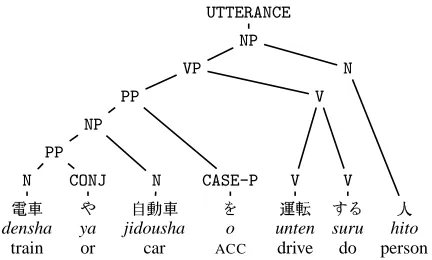
A (simplified) example of an entry is given in Fig-ure 1. Each entry contains the word itself, its part of speech, and its lexical type(s) in the grammar. Each sense then contains definition and example sentences, links to other senses in the lexicon (such as hypernym), and links to other resources, such as the Goi-Taikei Japanese Lexicon (Ikehara et al., 1997) and WordNet (Fellbaum, 1998). Each content word of the definition and example sentences is an-notated with sense tags from the same lexicon.

There were 4 parses for the definition sentence. The correct parse, shown as a phrase structure tree, is shown in Figure 2. The two sources of ambigu-ity are the conjunction and the relative clause. The parser also allows the conjunction to combine \

densha and 0 hito. In Japanese, relative clauses

can have gapped and non-gapped readings. In the gapped reading (selected here),0hito is the subject

ofþU unten “drive”. In the non-gapped reading

there is some underspecified relation between the modifee and the verb phrase. This is similar to the difference in the two readings of the day he knew in English: “the day that he knew about” (gapped) vs “the day on which he knew (something)” (non-gapped). Such semantic ambiguity is resolved by selecting the correct derivation tree that includes the applied rules in building the tree (Fig 3).

The semantic representation is Minimal Recur-sion Semantics (Copestake et al., 2005). We sim-plify this into a dependency representation, further abstracting away from quantification, as shown in Figure 4. One of the advantages of the HPSG sign is that it contains all this information, making it pos-sible to extract the particular view needed. In or-der to make linking to other resources, such as the sense annotation, easier predicates are labeled with pointers back to their position in the original sur-face string. For example, the predicatedensha n 1

links to the surface characters between positions 0 and 3:\.

UTTERANCE

NP

VP N

PP V

NP

PP

N CONJ N CASE-P V V

\ ℄ ¥ k þU 2d 0

densha ya jidousha o unten suru hito

train or car ACC drive do person

þU31“chauffeur”: “a person who drives a train or car”

Figure 2: Syntactic View of the Definition ofþU

31untenshu “chauffeur”

e2:unknown<0:13>[ARG x5:_hito_n] x7:densha_n_1<0:3>[]

x12:_jidousha_n<4:7>[]

x13:_ya_p_conj<0:4>[LIDX x7:_densha_n_1, RIDX x12:_jidousha_n] e23:_unten_s_2<8:10>[ARG1 x5:_hito_n] e23:_unten_s_2<8:10>[ARG2 x13:_ya_p_conj]

Figure 4: Simplified Dependency View of the Defi-nition ofþU31untenshu “chauffeur”

2.2 Semantic Annotation

The lexical semantic annotation uses the sense in-ventory from Lexeed (Kasahara et al., 2004). All words in the fundamental vocabulary are tagged with their sense. For example, the wordd&ookii

“big” (of example sentence in Figure 1) is tagged as sense 5 in the example sentence, with the meaning “elder, older”.

The word senses are further linked to semantic classes in a Japanese ontology. The ontology, Goi-Taikei, consists of a hierarchy of 2,710 semantic classes, defined for over 264,312 nouns, with a max-imum depth of 12 (Ikehara et al., 1997). We show the top 3 levels of the Goi-Taikei common noun on-tology in Figure 5. The semantic classes are prin-cipally defined for nouns (including verbal nouns), although there is some information for verbs and ad-jectives.

3 Parse Selection

can-

               

INDEX þU3 untenshu

POS noun

SENSE1



          

DEFINITION

h

\1℄¥1kþU12d04 a person who drives trains and cars

i

EXAMPLE

"

d&(5C<8b\1GþU31Dod6G%Ý32

I dream of growing up and becoming a train driver

#

HYPERNYM 04 hito “person”

SEM. CLASS h292:driveri(⊂ h4:personi) WORDNET motorman1



           

               

Figure 1: Dictionary Entry forþU31untenshu “chauffeur”

frag-np

rel-cl-sbj-gap

hd-complement noun-le

hd-complement v-light

hd-complement

hd-complement case-p-acc-le

noun-le conj-le noun-le vn-trans-le v-light-le

\ ℄ ¥ k þU 2d 0

densha ya jidousha o unten suru hito

train or car ACC drive do person

þU31“chauffeur”: “a person who drives a train or car”

Figure 3: Derivation Tree of the Definition ofþU31untenshu “chauffeur”

Phrasal nodes are labeled with identifiers of grammar rules, and (pre-terminal) lexical nodes with class names for types of lexical entries.

Lvl 0 Lvl 1 Lvl 2 Lvl 3

human agent organization

facility c

o n c r e t e

place region natural place object animate

inanimate abstract

thing mental state

noun action

human activity event phenomenon

natural phen. a

b s t r a c t

existence system relationship property relation state

shape amount location time

Figure 5: Top 3 levels of the GoiTaikei Ontology

didate analyses (for some Japanese string) according

to JACY, the goal is to rank parse trees by their prob-ability: training a stochastic parse selection model on the available treebank, we estimate statistics of various features of candidate analyses from the tree-bank. The definition and selection of features, thus, is a central parameter in the design of an effective parse selection model.

3.1 Syntactic Features

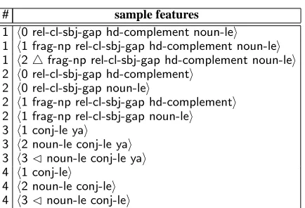
The first model that we trained uses syntactic fea-tures defined over HPSG derivation trees as summa-rized in Table 1. For the closely related purpose of parse selection over the English Redwoods treebank, Toutanova et al. (2005) train a discriminative log-linear model, using features defined over derivation

trees with non-terminals representing the construc-tion types and lexical types of the HPSG grammar.

deriva-# sample features

1 h0 rel-cl-sbj-gap hd-complement noun-lei

1 h1 frag-np rel-cl-sbj-gap hd-complement noun-lei

1 h2△frag-np rel-cl-sbj-gap hd-complement noun-lei

2 h0 rel-cl-sbj-gap hd-complementi

2 h0 rel-cl-sbj-gap noun-lei

2 h1 frag-np rel-cl-sbj-gap hd-complementi

2 h1 frag-np rel-cl-sbj-gap noun-lei

3 h1 conj-le yai

3 h2 noun-le conj-le yai

3 h3noun-le conj-le yai

4 h1 conj-lei

4 h2 noun-le conj-lei

4 h3noun-le conj-lei

Table 1: Example structural features extracted from the derivation tree in Figure 3. The first column numbers the feature template corresponding to each example; in the examples, the first integer value is a parameter to feature templates, i.e. the depth of grandparenting (types #1 and#2) or n-gram size (types #3 and #4). The special symbols △ and

denote the root of the tree and left periphery of the yield, respectively.

tion limited to depth one. Table 1 shows example features extracted from our running example (Fig-ure 3 above) in our MaxEnt models, where the fea-ture template #1 corresponds to local derivation sub-trees. We will refer to the parse selection model us-ing only local structural features asSYN-1.

3.1.1 Dominance Features

To reduce the effects of data sparseness, feature type #2 in Table 1 provides a back-off to deriva-tion sub-trees, where the sequence of daughters is reduced to just the head daughter. Conversely, to facilitate sampling of larger contexts than just sub-trees of depth one, feature template #1 allows op-tional grandparenting, including the upwards chain of dominating nodes in some features. In our ex-periments, we found that grandparenting of up to three dominating nodes gave the best balance of en-larged context vs. data sparseness. Enriching our ba-sic modelSYN-1with these features we will hence-forth callSYN-GP.

3.1.2 N-Gram Features

In addition to these dominance-oriented features taken from the derivation trees of each parse tree, our models also include more surface-oriented fea-tures, viz. n-grams of lexical types with or without

lexicalization. Feature type #3 in Table 1 defines

n-grams of variable size, where (in a loose

anal-ogy to part-of-speech tagging) sequences of lexical types capture syntactic category assignments. Fea-ture templates #3 and #4 only differ with regard to lexicalization, as the former includes the surface to-ken associated with the rightmost element of each

n-gram (loosely corresponding to the emission

prob-abilities in an HMM tagger). We used a maximum

n-gram size of two in the experiments reported here,

again due to its empirically determined best overall performance.

3.2 Semantic Features

In order to define semantic parse selection features, we use a reduction of the full semantic representa-tion (MRS) into ‘variable-free’ elementary

depen-dencies. The conversion centrally rests on a notion

of one distinguished variable in each semantic rela-tion. For most types of relations, the distinguished variable corresponds to the main index (ARG0in the examples above), e.g. an event variable for verbal re-lations and a referential index for nominals. Assum-ing further that, by and large, there is a unique re-lation for each semantic variable for which it serves as the main index (thus assuming, for example, that adjectives and adverbs have event variables of their own, which can be motivated in predicative usages at least), an MRS can be broken down into a set of basic dependency tuples of the form shown in Fig-ure 4 (Oepen and Lønning, 2006).

All predicates are indexed to the position of the word or words that introduced them in the input sen-tence (<start:end>). This allows us to link them to the sense annotations in the corpus.

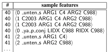
3.2.1 Basic Semantic Dependencies

The basic semantic model, SEM-Dep, consists of features based on a predicate and its arguments taken from the elementary dependencies. For example, consider the dependencies for densha ya

jidousha-wo unten suru hito “a person who drives a train or

car” given in Figure 4. The predicate unten “drive” has two arguments: ARG1 hito “person” and ARG2

jidousha “car”.

# sample features

20 h0 unten s ARG1 hito n 1 ARG2 ya p conji

20 h0 ya p conj LIDX densha n 1 RIDX jidousha n 1i

21 h1 unten s ARG1 hito n 1i

21 h1 unten s ARG2 jidousha n 1i

21 h1 ya p conj LIDX densha n 1i

21 h1 ya p conj RIDX jidousha n 1i

22 h2 unten s hito n 1 jidousha n 1i

23 h3 unten s hito n 1i

23 h3 unten s jidousha n 1i

. . .

Table 2: Example semantic features (SEM-Dep) ex-tracted from the dependency tree in Figure 4.

only one argument at a time, #22 provides unlabeled relations, #23 provides one unlabeled relation at a time and so on.

Each combination of a predicate and its related argument(s) becomes a feature. These resemble the basic semantic features used by Toutanova et al. (2005). We further simplify these by collapsing some non-informative predicates, e.g. theunknown

predicate used in fragments.

3.2.2 Word Sense and Semantic Class Dependencies

We created two sets of features based only on the word senses. ForSEM-WSwe used the sense anno-tation to replace each underspecified MRS predicate by a predicate indicating the word sense. This used the gold standard sense tags. ForSEM-Class, we used the sense annotation to replace each predicate by its Goi-Taikei semantic class.

In addition, to capture more useful relationships, conjunctions were followed down into the left and right daughters, and added as separate features. The semantic classes for \1densha “train” and ¥

1jidousha “car” are both h988:land vehiclei,

while þU1 unten “drive” is h2003:motioni and

04hito “person”ish4:humani. The sample features

ofSEM-Classare shown in Table 3.

These features provide more specific information, in the case of the word sense, and semantic smooth-ing in the case of the semantic classes, as words are binned into only 2,700 classes.

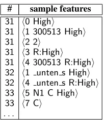
3.2.3 Superordinate Semantic Classes

We further smooth these features by replacing the semantic classes with their hypernyms at a given level (SEM-L). We investigated levels 2 to 5.

Pred-# sample features

40 h0 unten s ARG1 C4 ARG2 C988i

40 h1 C2003 ARG1 C4 ARG2 C988i

40 h1 C2003 ARG1 C4 ARG2 C988i

40 h0 ya p conj LIDX C988 RIDX C988i

41 h2 unten s ARG1 C4i

41 h2 unten s ARG2 C988i

. . .

Table 3: Example semantic class features (

SEM-Class).

icates are binned into only 9 classes at level 2, 30 classes at level 3, 136 classes at level 4, and 392 classes at level 5.

For example, at level 3, the hypernym class for h988:land vehiclei is h706:inanimatei,

h2003:motioni is h1236:human activityi

and h4:humani is unchanged. So we used

h706:inanimatei and h1236:human activityi

to make features in the same way as Table 3. An advantage of these underspecified semantic classes is that they are more robust to errors in word sense disambiguation — fine grained sense distinc-tions can be ignored.

3.2.4 Valency Dictionary Compatability

The last kind of semantic information we use is valency information, taken from the Japanese side of the Goi-Taikei Japanese-English valency dictio-nary as extended by Fujita and Bond (2004).This va-lency dictionary has detailed information about the argument properties of verbs and adjectives, includ-ing subcategorization and selectional restrictions. A simplified entry of the Japanese side for þU2

dunten-suru “drive” is shown in Figure 6.

Each entry has a predicate and several case-slots. Each case-slot has information such as grammatical function, case-marker, case-role (N1, N2, . . . ) and semantic restrictions. The semantic restrictions are defined by the Goi-Taikei’s semantic classes.

On the Japanese side of Goi-Taikei’s valency dictionary, there are 10,146 types of verbs giving 18,512 entries and 1,723 types of adjectives giving 2,618 entries.

The valency based features were constructed by first finding the most appropriate pattern, and then recording how well it matched.

PID:300513

” N1 <4:people> "%" ga ˜ N2 <986:vehicles> "k" o

— þU2d unten-suru

Figure 6: þU2dunten-suru “N1 drive N2”.

PID is the verb’s Pattern ID

# sample features

31 h0 Highi

31 h1 300513 Highi

31 h2 2i

31 h3 R:Highi

31 h4 300513 R:Highi

32 h1 unten s Highi

32 h4 unten s R:Highi

33 h5 N1 C Highi

33 h7 Ci

. . .

Table 4: Example semantic features (SP)

same as the predicate in the sentence: for exam-ple we look up all entries for þU2d

unten-suru “drive”. Then, for each candidate pattern, we

mapped its arguments to the target predicate’s ar-guments via case-markers. If the target predicate has no suitable argument, we mapped to comitative phrase. Finally, for each candidate patterns, we cal-culate a matching score1and select the pattern which has the best score.

Once we have the most appropriate pattern, we then construct features that record how good the match is (Table 4). These include: the to-tal score, with or without the verb’s Pattern ID (High/Med/Low/Zero: #31 0,1), the number of filled arguments (#31 2), the fraction of filled arguments vs all arguments (High/Med/Low/Zero: #31 3,4), the score for each argument of the pattern (#32 5) and the types of matches (#32 5,7).

These scores allow us to use information about word usage in an exisiting dictionary.

4 Evaluation and Results

We trained and tested on a subset of the dictionary definition and example sentences in the Hinoki cor-pus. This consists of those sentences with ambigu-ous parses which have been annotated so that the

1_{The scoring method follows Bond and Shirai (1997), and}

depends on the goodness of the matches of the arguments.

number of parses has been reduced (Table 5). That is, we excluded unambiguous sentences (with a sin-gle parse), and those where the annotators judged that no parse gave the correct semantics. This does not necessarily mean that there is a single correct parse, we allow the annotator to claim that two or more parses are equally appropriate.

Corpus # Sents Length Parses/Sent (Ave) (Ave) Definitions Train 30,345 9.3 190.1 Test 2,790 10.1 177.0 Examples Train 27,081 10.9 74.1 Test 2,587 10.4 47.3

Table 5: Data of Sets for Evaluation

Dictionary definition sentences are a different genre to other commonly used test sets (e.g news-paper text in the Penn Treebank or travel dialogues in Redwoods). However, they are valid examples of naturally occurring texts and a native speaker can read and understand them without special training. The main differences with newspaper text is that the definition sentences are shorter, contain more fragments (especially NPs as single utterances) and fewer quoting and proper names. The main differ-ences with travel dialogues is the lack of questions.

4.1 A Maximum Entropy Ranker

Log-linear models provide a very flexible frame-work that has been widely used for a range of tasks in NLP, including parse selection and reranking for machine translation. We use a maximum entropy

/ minimum divergence (MEMD) modeler to train

the parse selection model. Specifically, we use the open-source Toolkit for Advanced Discriminative

Modeling (TADM:2 Malouf, 2002) for training, us-ing its limited-memory variable metric as the opti-mization method and determining best-performing convergence thresholds and prior sizes experimen-tally. A comparison of this learner with the use of support vector machines over similar data found that the SVMs gave comparable results but were far slower (Baldridge and Osborne, 2007). Because we are investigating the effects of various different fea-tures, we chose the faster learner.

Method Definitions Examples Accuracy Features Accuracy Features

(%) (×1000) (%) (×1000)

SYN-1 52.8 7 67.6 8

SYN-GP 62.7 266 76.0 196

SYN-ALL 63.8 316 76.2 245

SYNbaseline 16.4 random 22.3 random

SEM-Dep 57.3 1,189 58.7 675

+SEM-WS 56.2 1,904 59.0 1,486

+SEM-Class 57.5 2,018 59.7 1,669

+SEM-L2 60.3 808 62.9 823

+SEM-L3 59.8 876 62.8 879

+SEM-L4 59.9 1,000 62.3 973

+SEM-L5 60.4 1,240 61.3 1,202

+SP 59.1 1,218 68.2 819

+SEM-ALL 62.7 3,384 69.1 2,693

SYN-SEM 69.5 2,476 79.2 2,126

SEMbaseline 20.3 random 22.8 random

Table 6: Parse Selection Results

4.2 Results

The results for most of the models discussed in the previous section are shown in Table 6. The accuracy is exact match for the entire sentence: a model gets a point only if its top ranked analysis is the same as an analysis selected as correct in Hinoki. This is a stricter metric than component based measures (e.g., labelled precision) which award partial credit for in-correct parses. For the syntactic models, the base-line (random choice) is 16.4% for the definitions and 22.3% for the examples. Definition sentences are harder to parse than the example sentences. This is mainly because they have fewer relative clauses and coordinate NPs, both large sources of ambigu-ity. For the semantic and combined models, multiple sentences can have different parses but the same se-mantics. In this case all sentences with the correct semantics are scored as good. This raises the base-lines to 20.3 and 22.8% respectively.

Even the simplest models (SYN-1 and SEM-Dep) give a large improvement over the baseline. Adding grandparenting to the syntactic model has a large improvement (SYN-GP), but adding lexical n-grams gave only a slight improvement over this (SYN-ALL). The effect of smoothing by superordinate seman-tic classes (SEM-Class), shows a modest improve-ment. The syntactic model already contains a back-off to lexical-types, we hypothesize that the seman-tic classes behave in the same way. Surprisingly, as we add more data, the very top level of the seman-tic class hierarchy performs almost as well as the

+

+ + +

+ + ₊ + + + +

b

c

b

c bc bc

b

c bc bc bc bc bc bc

l d

l d ld ld

l

d ld ld ld ld l d ld

0 20 40 60 80 100

20 30 40 50 60 70

% of training data (30,345 sentences)

S

en

t.

A

cc

u

ra

cy SYN-SEM

SEM-ALL SYN-ALL

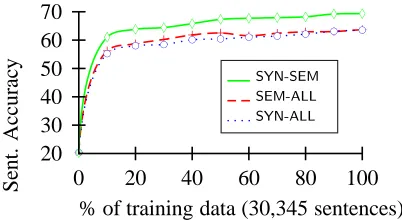
Figure 7: Learning Curves (Definitions)

more detailed levels. The features using the valency dictionary (SP) also provide a considerable improve-ment over the basic dependencies.

Combining all the semantic features (SEM-ALL) provides a clear improvement, suggesting that the information is heterogeneous. Finally, combing the syntactic and semantic features gives the best results by far (SYN-SEM:SYN-ALL+SEM-Dep+SEM-Class+

SEM-L2 +SP). The definitions sentences are harder

syntactically, and thus get more of a boost from the semantics. The semantics still improve performance for the example sentences.

The semantic class based sense features used here are based on manual annotation, and thus show an upper bound on the effects of these features. This is not an absolute upper bound on the use of sense information — it may be possible to improve further through feature engineering. The learning curves (Fig 7) have not yet flattened out. We can still im-prove by increasing the size of the training data.

5 Discussion

Pioneering work by Toutanova et al. (2005) and Baldridge and Osborne (2007) on parse selection for an English HPSG treebank used simpler semantic features without sense information, and got a far less dramatic improvement when they combined syntac-tic and semansyntac-tic information.

The use of hand-crafted lexical resources such as the Goi-Taikei ontology is sometimes criticized on the grounds that such resources are hard to produce and scarce. While it is true that valency lexicons and sense hierarchies are hard to produce, they are of such value that they have already been created for all of the languages we know of which have large treebanks. In fact, there are more languages with WordNets than large treebanks.

In future work we intend to confirm that we can get improved results with raw sense disambiguation results not just the gold standard annotations and test the results on other sections of the Hinoki corpus.

6 Conclusions

We have shown that sense-based semantic features combined with ontological information are effec-tive for parse selection. Training and testing on the definition subset of the Hinoki corpus, a com-bined model gave a 5.6% improvement in parse se-lection accuracy over a model using only syntactic features (63.8% →69.4%). Similar results (76.2%

→79.2%) were found with example sentences.

References

Jason Baldridge and Miles Osborne. 2007. Active learning and logarithmic opinion pools for HPSG parse selection. Natural

Language Engineering, 13(1):1–32.

Daniel M. Bikel. 2000. A statistical model for parsing and word-sense disambiguation. In Proceedings of the Joint

SIG-DAT Conference on Empirical Methods in Natural Language Processing and Very Large Corpora, pages 155–163. Hong

Kong.

Francis Bond, Sanae Fujita, and Takaaki Tanaka. 2007. The Hi-noki syntactic and semantic treebank of Japanese. Language

Resources and Evaluation. (Special issue on Asian language

technology).

Francis Bond and Satoshi Shirai. 1997. Practical and efficient organization of a large valency dictionary. In Workshop on

Multilingual Information Processing — Natural Language Processing Pacific Rim Symposium ’97: NLPRS-97. Phuket.

Ann Copestake, Dan Flickinger, Carl Pollard, and Ivan A. Sag. 2005. Minimal Recursion Semantics. An introduction.

Re-search on Language and Computation, 3(4):281–332.

Christine Fellbaum, editor. 1998. WordNet: An Electronic

Lex-ical Database. MIT Press.

Sanae Fujita and Francis Bond. 2004. A method of creating new bilingual valency entries using alternations. In Gilles S´erasset, editor, COLING 2004 Multilingual Linguistic

Re-sources, pages 41–48. Geneva.

Eduard Hovy, Mitchell Marcus, Martha Palmer, Lance Ramshaw, and Ralph Weischedel. 2006. Ontonotes: The 90% solution. In Proceedings of the Human Language

Technology Conference of the NAACL, Companion Volume: Short Papers, pages 57–60. Association for Computational

Linguistics, New York City, USA. URL http://www. aclweb.org/anthology/N/N06/N06-2015.

Satoru Ikehara, Masahiro Miyazaki, Satoshi Shirai, Akio Yokoo, Hiromi Nakaiwa, Kentaro Ogura, Yoshifumi Ooyama, and Yoshihiko Hayashi. 1997. Goi-Taikei — A Japanese Lexicon. Iwanami Shoten, Tokyo. 5 vol-umes/CDROM.

Kaname Kasahara, Hiroshi Sato, Francis Bond, Takaaki Tanaka, Sanae Fujita, Tomoko Kanasugi, and Shigeaki Amano. 2004. Construction of a Japanese semantic lexicon: Lexeed. In IPSG SIG: 2004-NLC-159, pages 75–82. Tokyo. (in Japanese).

Dan Klein and Christopher D. Manning. 2003. Accurate un-lexicalized parsing. In Erhard Hinrichs and Dan Roth, edi-tors, Proceedings of the 41st Annual Meeting of the

Associ-ation for ComputAssoci-ational Linguistics, pages 423–430. URL

http://www.aclweb.org/anthology/P03-1054.pdf. Robert Malouf. 2002. A comparison of algorithms for

maxi-mum entropy parameter estimation. In CONLL-2002, pages 49–55. Taipei, Taiwan.

Robert Malouf and Gertjan van Noord. 2004. Wide cover-age parsing with stochastic attribute value grammars. In

IJCNLP-04 Workshop: Beyond shallow analyses - For-malisms and statistical modeling for deep analyses. JST

CREST. URLhttp://www-tsujii.is.s.u-tokyo.ac. jp/bsa/papers/malouf.pdf.

Stephan Oepen, Dan Flickinger, Kristina Toutanova, and Christoper D. Manning. 2004. LinGO redwoods: A rich and dynamic treebank for HPSG. Research on Language and

Computation, 2(4):575–596.

Stephan Oepen and Jan Tore Lønning. 2006. Discriminant-based MRS banking. In Proceedings of the 5th International

Conference on Language Resources and Evaluation (LREC 2006). Genoa, Italy.

Carl Pollard and Ivan A. Sag. 1994. Head Driven Phrase

Struc-ture Grammar. University of Chicago Press, Chicago.

Melanie Siegel and Emily M. Bender. 2002. Efficient deep pro-cessing of Japanese. In Proceedings of the 3rd Workshop on

Asian Language Resources and International Standardiza-tion at the 19th InternaStandardiza-tional Conference on ComputaStandardiza-tional Linguistics, pages 1–8. Taipei.

Kristina Toutanova, Christopher D. Manning, Dan Flickinger, and Stephan Oepen. 2005. Stochastic HPSG parse disam-biguation using the redwoods corpus. Research on Language

and Computation, 3(1):83–105.

Deyi Xiong, Qun Liu Shuanglong Li and, Shouxun Lin, and Yueliang Qian. 2005. Parsing the Penn Chinese treebank with semantic knowledge. In Robert Dale, Jian Su Kam-Fai Wong and, and Oi Yee Kwong, editors, Natural Language