2777
Parallel Frequent Pattern Mining to Alleviate the
Computational Snags in Very Large Datasets Using
Divide and Conquer Approach
M.Uma1, Dr.V.Baby Deepa2
Ph.D. Research Scholar(P.T.), PG and Research Department of Computer Science, Government Arts College (Autonomous), Karur-639 005. 1
Assistant Professor, PG and Research Department of Computer Science, Government Arts College(Autonomous),, Karur-639 005. 2
Email : [email protected]1, [email protected]2
Abstract- The frequent mining is not a new area to explore and lot of research works are carried out by many authors but still the FIM is subject to some improvement when dealt with very large datasets. This paper deals with very large dataset and utilizes divide and conquer approach (i.e.) partition the dataset into many parts and process the mining task to reduce the burden related to time complexity and memory consumption. The proposed approach uses bit vector representation and the local support is initially calculated for the partitioned datasets using parallel computation on several processors and then the k- found is merged together to find the global support. Now the merged data is again partitioned to find the k+1 local support using parallel processing and the merged back to find the global support. This divide and merge process is continued until the size of the merged data becomes smaller for computation. Here the unpromising items are pruned and the final resultant is portrayed and the time and memory footprints are calculated for the datasets. From the experimental result it is quite clear that the parallelism inducted in this paper reduces the time and increases the speed considerably when executed on very large datasets.
Index Terms: Big Data, Frequent Mining, Item sets, Divide and Conquer
1. INTRODUCTION
The foremost objective of the data mining is to unearth inherent, hidden, and useful information from the large raw data [1]. Frequent mining is one of the most regularly used data mining process which discovers frequently co-occurring items, incidents, or objects (e.g., frequently bought items in shops). One of the most famous frequent pattern mining algorithms is the Apriori algorithm [6] proposed by Aggarwal and Srikant which employs a generate-and-test approach in discovering frequent patterns level-wise and bottom-up technique. In other words, the algorithm first generates candidate patterns of cardinality k (i.e., candidate k-s) and tests if each of them is frequent (i.e., tests if its support or frequency meets or exceeds the user-specified minimum support threshold). Then the algorithm generates k+1 item set which satisfies the minimum support and continues to generate until all the frequent item sets are found.
The FP-Growth algorithm [2] is another well-known frequent pattern mining algorithm. It
utilizes an expanded prefix-tree structure called a Frequent Pattern Tree (FP-tree) to catch the core of the database. FP-Growth unlike Apriori which checks the database K times (where K is the greatest cardinality of the found frequent patterns), FP-growth scans the database only twice. The important concept of FP-Growth is to recursively obtain applicable paths from the FP-tree to frame projected databases (i.e., accumulations of transactions containing a few items), from which sub-trees (i.e., small FP-trees) catching the content of important transactions produced.
2778
Big Data
The main goal of the paper was to apply the proposed algorithm to mine big data using partitioning technique. Big data [3], [5] are present in all areas and verticals. Usually they are high veracity, velocity, value, variety and volume past the capacity of usually utilized programming to oversee, query, and process at low time. These high volumes of profitable data can be effectively gathered or produced at a high velocity from various data sources (which may prompt diverse data formats) in different genuine applications, for example, bioinformatics, click streams, market basket data, social network, and additionally from the internet [4].
Features Of Big Data
The following are the main characteristics of the big data, and they are illustrated by 5V’s,
Veracity-emphases on the quality of the input raw data (e.g., doubtfulness, disorder, andcredibility of the data)
Velocity–the speed at which data are archived or
discovered.
Value- the usefulness of data.
Variety- various types, contents or formats of data.
Volume- focuses on the quantity of data.
Due to the 5Vs" attributes of big data, new types of algorithm are required for overseeing, querying, and processing these big data in order to empower improved basic leadership, understanding, and process enhancement. This imbues and spurs research and practices in data science, which intend to create orderly or quantitative data analytic algorithms to examine (e.g., assess, clean, change, and model) and mine big data.
[image:2.595.65.532.382.624.2]2. PROPOSED APPROACH
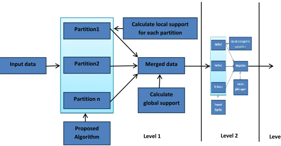
Figure 1: Proposed approach The proposed approach or the architecture
is shown in the figure 1. The input raw data is initially fed and as the size of the input data is too large, the architecture apportioning layer divides the data and each of the data is processed in parallel. Here the proposed algorithm is applied and the local support count is found. The processed itemsets are then merged together and here the data
compression takes place using grouping of the similar with the number of occurrences global support value (gS). This will considerably reduce the size of the merged data.
M-data ={, gS}. Suppose itemset {A, B} is found in 1289 transactions, the M-data itemset = {(A, B),1289}
Input data
Partition1
Partition2
Partition n
Proposed Algorithm
Merged data Calculate local support
for each partition
Calculate global support
2779 The merged and compressed data is again
partitioned to split the data into smaller parts and the parallel processing takes place to find the local support and then merged to find the global support. This process is continued until the merged dataset size becomes smaller enough to process without parallel computing.
3.PROPOSED ALGORITHM
The proposed algorithm starts with the discovery of unique items present in the partitioned data. This procedure clearly finds the distinct item present with the frequency. Once the unique items are found the bit vector representation is carried out to denote whether the item is present in the transaction or not. If present it is marked by the bit
value “1” else marked by the bit value “0”. Initially in the level 1, the two candidates are formed using the bit vector table and using simple AND operation to find the number of occurrences (local support value-LSV). The different processor processed and discovered 2-itemsrts are merged together to find the global support and then the data compression is carried out using grouping the similar and representing the data in {,gS} format. Here if the global count of the item sets which are less than the user specified minimum support threshold value are pruned away and the unpromising items are removed from the merged to reduce the size of the merged data considerably. The same process is continued until the data becomes small enough to process in a single processor.
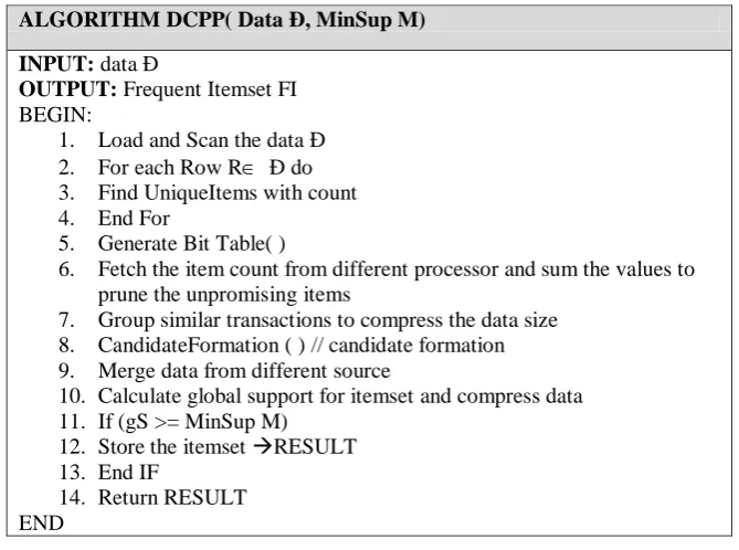
3.1 Divide And Conquer Parallel Processing Algorithm
ALGORITHM DCPP( Data Ð, MinSup M)
INPUT: data Ð
OUTPUT: Frequent Itemset FI
BEGIN:
1. Load and Scan the data Ð 2. For each Row R Ð do 3. Find UniqueItems with count 4. End For
5. Generate Bit Table( )
6. Fetch the item count from different processor and sum the values to prune the unpromising items
7. Group similar transactions to compress the data size 8. CandidateFormation ( ) // candidate formation 9. Merge data from different source
10. Calculate global support for itemset and compress data 11. If (gS >= MinSup M)
12. Store the itemset RESULT 13. End IF
[image:3.595.114.449.323.572.2]14. Return RESULT END
Figure 2: Pseudo code of the DCPP algorithm
The proposed algorithm is explained with a sample dataset for clear understanding and the table 1 shows the sample dataset.
Table 1: Sample dataset
TID ITEMS
T1 1, 2, 3, 5, 6, 15
T2 1, 3, 7
T3 5, 9
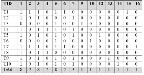
2780 The initial step of finding the unique items is performed and there are 14 different items present in the sample dataset comprising of 10 transactions. Scan the dataset and then the bit table is constructed according to the items presence as shown in the figure 3.
Figure 3: Bit table construction for the sample dataset
PROCEDURE generateBIT-Table( Database Ð) INPUT: database Ð
OUTPUT: Bit table BEGIN:
1. Load and Scan the data Ð 2. For each Row R Ð do 3. If (UniqueItem present in R) 4. Mark “1” in bit table 5. Else
6. Mark “0” in bit table 7. End if
8. End For 9. Return bit table END
Figure 4: Pseudo code to generate bit table The pseudo code to generate the bit table
is shown in the figure 4 and the generated table is shown in the figure 3. The count from the various processors is fetched and then the single items with less minimum support values are removed. The next process is to form the candidates along with the local support count. Let us assume that the user
defined support threshold value is given to be 2. Here the 1-itemset count is fetched from different processor to make sure that the promising items should not be pruned away locally. Here assume that the items {9,10,12,13,14,15,16} fetched from the other processors have lower support count and hence pruned away locally.
T5 1,3,5,7,12
T6 5, 10
T7 1,2,3,5,6, 16
T8 1,3,4
T9 1,3,5,7,13
[image:4.595.179.423.260.387.2]2781 Figure 5: Frequent 1-itemset
The data compression in the form of grouping the similar items are carried out and the transactions with 10 rows are reduced to 6 rows after the compression and hence the size of the
dataset is reduced to almost 40%. The number of times the transaction (TC) occurs is noted to form the candidates in the next step.
Figure 6: Compressed dataset Actually the sample dataset shown in the table 1 is partitioned into two parts (i.e.) transactions [1-5] and transactions [6-10] are bifurcated to facilitate the speed of the execution
and to reduce the memory consumption. But for brevity, the entire transaction is taken as a partition and processed as example.
PROCEDURE candidateFormation( Bit table, Unique items) INPUT: Bit table, Unique Items
OUTPUT: Candidates with local support count BEGIN:
1. For i1to UniqueItemCount do 2. For j [i+1] to UniqueItemCount do 3. CUniqueItem[i] UniqueItem[j]
4. Fetch the bit table to calculate support using AND operation 5. Store Res {C, support count}
6. Store pruned candidates in P-Res to find whether the candidate is really worthy when merged with other partitions.
7. End For 8. End For
[image:5.595.179.443.100.245.2]9. Return Res, P-Res END PROCEDURE
Figure 7: Pseudo code to generate local candidates ITEMS
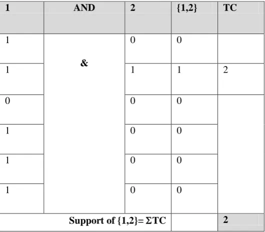
[image:5.595.222.376.348.468.2]2782 Here the items “1” and “2” is initially
formed by the union operation and the support count is computed from the bit table. The item “1”
[image:6.595.166.431.162.394.2]and item “2” columns are fetched to perform the AND operation to find the exact frequency of the {1, 2} s shown below,
Figure 8: calculation of the count and candidate formation Here the compressed dataset is considered
and the presence of the 1’s in the both items is checked by using simple AND operation and the TC value corresponding to the items with 1’s are summed to get the local support count. Since the occurrence of {1, 2} is TRUE only in one occasion
as shown in the figure 8 (row 2) the corresponding TC=2 is taken and the support count of {1,2}= 2. Similarly all the candidates are formed and the candidate along with the local support count {(1, 2), 2}is archived in the result to be merged for global support computations.
PROMISING ITEMS – (Res) UNPROMISING ITEMS – (P-Res)
2 ITEMSET Count 2 ITEMSET COUNT
1,2 2 2,4 0
1,3 8 2,7 0
1,4 2 4,6 0
1,5 6 4,5 1
1,6 2 4,7 1
2,3 2
2,5 2
2,6 2
3,4 2
3.5 6
3,6 2
3,7 5
5,6 2
5,7 4
Figure 9: First level local candidates formed from one processor
1 AND 2 {1,2} TC
1
&
0 0
1 1 1 2
0 0 0
1 0 0
1 0 0
1 0 0
2783 Now the partitioned candidates generated
from various processors are merged into a single dataset to calculate the global support and if the global support is found to be higher than or equal to the user defined support threshold value, the
resultant candidates are stored in result. And the unpromising candidates are pruned and then again this merged dataset is partitioned and recursively executed to form the next (k+1) candidates using the DCPP algorithm.
3.2 Property 1
A global frequent itemset {(X,Y), gS} may not be a local frequent itemset {(X,Y),LSC}.
{(X,Y), gS} ≠ {(X,Y),LSC}
3.3 Property 2
An itemset which may appear infrequent in one partition may be frequent in another partition or may be frequent in the global merged dataset.
3.4 Property 3
Given a large dataset which comprises of n partitions where the minimum support count is M, the global frequent item set Cn may or may not appear in the partitions Ci, i=1,2,3,…n
4. EXPERIMENTAL RESULTS
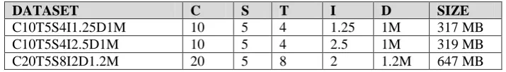
[image:7.595.80.484.400.477.2]Experiments are carried out to test the performance of the proposed algorithm using very large synthetic dataset and the coding is done using C#.NET. For the experimental purpose 10 nodes are utilized and all the systems configuration is Intel Core I7 processor with 4GB RAM and 2TB HDD. The synthetic dataset are generated by the IBM Quest data mining code [7].The parameters of the dataset are shown in the table 2.
Table 2: Parameters used in synthetic dataset generation
4.1
Dataset Used
Table 3: Synthetic dataset used for experiment
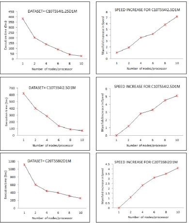
The execution time for the proposed algorithm is computed with a fixed support value for each dataset and using various numbers of processors to check the running time and the increase in speed of the DCPP algorithm. The
minimum support values for the first dataset provided = 0.25, for the second dataset = 0.3 and for the third large dataset=0.45. The execution time and the increase in the speed are shown in the figure 9 for all the datasets.
Parameters Description of parameter
D Total number of sequences in the dataset C Average number of transactions per sequence T Average number of items per transaction S Average length of maximal sequence.
I Average length of transactions within the maximal sequences
DATASET C S T I D SIZE
[image:7.595.174.532.532.583.2]2784 The figure 10 portrays the total execution
time for the datasets and the increase in the speed of execution when the number of processor is increased and from the figures the speed of the execution is increased 2 times when two nodes or processors are employed. When the node size or the processor is increased to 6, the speed increased to almost 3.8 times. When the maximum number of nodes is employed the speed increased approximately 6-7 times which is actually a good
[image:8.595.82.473.238.699.2]performance when the parallel and partitioned approach is utilized with divide and conquers technique. The execution time too reduces sharply when the number of processor increases and the proposed algorithm can handle dataset exceeding 10 – 15 GB.
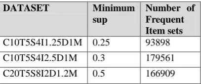
2785 The number of frequent item set found is
[image:9.595.69.273.217.302.2]also calculated and displayed in the table 4. The large synthetic datasets used in the experiment produced huge volume of frequent item sets which is practically impossible to be generated by the single processor at the speed at which the parallel divide and conquer approach discovered.
Table 4: Frequent item sets discovered
Table 4: Frequent item sets discovered
DATASET Minimum
sup
Number of Frequent Item sets
C10T5S4I1.25D1M 0.25 93898 C10T5S4I2.5D1M 0.3 179561 C20T5S8I2D1.2M 0.5 166909
5. CONCLUSION AND FUTURE SCOPE
The proposed DCPP algorithm performed reasonably well and with the increase in the number of nodes the performance related to the time also increases proportionately. Since the proposed algorithm employs level wise partitioning technique, the pruning is also carried out effectively to reduce the memory consumption and the compression technique utilized decreases the size of the dataset considerably. This proposed algorithm in future can be employed using map reduce to improve the overall performance further.
REFERENCES
[1] Rakesh Agrawal, Tomasz Imieli nski, and Arun Swami. Mining association rules between sets of items in large databases. In Proceedings of the 1993 ACM SIGMOD International Conference on Management of Data (SIGMOD 1993), Washington, DC, USA, pages 207{216. ACM, 1993.
[2] Jiawei Han, Jian Pei, and Yiwen Yin. Mining frequent patterns without candidate generation. SIGMOD Records, 29(2):1{12, May 2000. [3] Alfredo Cuzzocrea, Domenico Sacc a, and
Je rey D. Ullman. Big data: A research agenda. In Proceedings of the 17th International Database Engineering & Applications Symposium (IDEAS 2013), Barcelona, Spain, pages 198{203. ACM, 2013.
[4] Alfredo Cuzzocrea, Ladjel Bellatreche, and Il-Yeol Song. Data warehousing and olap over
big data: Current challenges and future research directions. In Proceedings of the 16th International Workshop on Data Warehousing and OLAP (DOLAP 2013), San Francisco, California, USA, pages 67-70. ACM, 2013. [5] Arun Kejariwal. Big data challenges: A
program optimization perspective. In Proceedings of the 2nd International Conference on Cloud and Green Computing (CGC 2012), Xiangtan, China, pages 702{707. IEEE Computer Society, 2012.
[6] Rakesh Agrawal and Ramakrishnan Srikant. Fast algorithms for mining association rules in large databases. In Proceedings of the 20th International Conference on Very Large Data Bases (VLDB 1994), Santiago de Chile, Chile, pages 487{499. Morgan Kaufmann Publishers Inc., 1994.
[7]QuestData Mining Project, available at http: www.almaden.ibm.com/
cs/quest/syndata.html., IBM Almaden Research Center, San Jose, CA 95120.
[8] M. J. Zaki, S. Parthasarathy, M. Ogihara, and W. Li, Parallel algorithms for fast discovery of association rules, Data Mining Knowledge Discovery 1, 4 (December 1997), 343 373. [9]M.-Y. Lin, P.-Y. Lee, and S.-C. Hsueh.
![table 1 is partitioned into two parts (i.e.) Actually the sample dataset shown in the transactions [1-5] and transactions [6-10] are bifurcated to facilitate the speed of the execution PROCEDURE candidateFormation( Bit table, Unique items)](https://thumb-us.123doks.com/thumbv2/123dok_us/737584.1083675/5.595.222.376.348.468/partitioned-transactions-transactions-bifurcated-facilitate-execution-procedure-candidateformation.webp)