Volume 4, No. 11, Nov-Dec 2013
International Journal of Advanced Research in Computer Science
RESEARCH PAPER
Available Online at www.ijarcs.info
Improvements on Heuristic Algorithms for Solving Traveling Salesman Problem
Fidan Nuriyeva Institute of Cybernetics
Azerbaijan National Academy of Sciences Baku, Azerbaijan
Gözde Kızılateş Department of Mathematics Faculty of Science, Ege University
Izmir, Turkey [email protected]
Murat Erşen Berberler Department of Computer Science Faculty of Science, Dokuz Eylul University
Izmir, Turkey [email protected]
Abstract: In this paper, four new heuristics are proposed in order to solve the traveling salesman problem. Comparisons are made between the results obtained from those heuristics. A new version of 2-opt and 3-opt methods are developed namely as 2-opt + 3-opt Shifting method. In addition, a new hybrid algorithm based on NN and Greedy algorithms is proposed. Computational experiments and comparisons are made on
library problems for Hybrid, NN, and Greedy algorithms. Obtained results show the efficiency of the algorithms.
Keywords: Traveling salesman problem; heuristic algorithms; hyper-heuristic algorithms; hybrid algorithms
I. INTRODUCTION
The traveling salesman problem (TSP) is a well-known and important combinatorial optimization problem [11]. The goal is to find the shortest (least expensive) tour that visits each city (node) in a given list exactly once and then returns to the starting city. In other words, TSP can be considered as a graph problem in which vertices represent cities and distances between cities are represented by edges.
Formally, the TSP can be stated as follows: The distances between n cities are stored in a distance matrix D with elements
d
ij wherei j
,
=
1,...,
n
and the diagonalelements
d
ii are zero. A tour can be represented by a cyclicpermutation
π
of{1, 2,..., }
n
whereπ
i represents the citythat follows city
i
on the tour. The traveling salesman problem is then the optimization problem of finding a permutationπ
that minimizes the length of the tour denotedby 1
( )
ni i
d
π
i
=
∑
.In this paper we shall concentrate on the symmetric TSP, in which the distances satisfy
d i j
( , )
=
d j i
( , )
for1
≤
i j
,
≤
n
.There are many variations of TSP: Symmetric TSP, Asymmetric TSP, The MAX TSP, The MIN TSP, TSP with multiple visits (TSPM), TSP with a closed tour, TSP with an open tour [3]. There are many variations of the problem. In this work, we examine the classic symmetric TSP.
Solving TSP is an important part of many applications in different fields including vehicle routing, computer wiring, machine sequencing and scheduling, frequency assignment in communication networks as well as data analysis in psychology and clustering in biostatistics [12, 17]. For
example, data analysis applications in psychology ranging from profile smoothing to finding an order in developmental data are presented by [5]. Clustering and ordering using TSP solvers are currently becoming popular in biostatistics [2, 13]. For example, [18] described an application for ordering genes and [9] used a TSP solver for clustering proteins.
Given that the problem is NP-Hard, and hence the polynomial-time algorithms for finding optimal tours are unlikely to exist, much attention has been addressed to the question of efficient heuristic algorithms, fast algorithms that attempt only to find near-optimal tours.
The rest of this paper is organized as follows. Section 2 describes some approaches for solving the TSP. Section 3 presents basic tour constructing algorithms such as NN and Greedy. Section 4 presents our new tour constructing proposed heuristics. Section 5 presents a new version of 2-opt and 3-2-opt algorithms that we have proposed. Section 6 presents other improved algorithms. Finally, section 7 concludes the paper.
II. APPROACHESFORSOLVINGTSP
Although definition of the TSP is easy, it belongs to NP-hard [6]. There are a number of algorithms used to find optimal tours, because of this problem is NP-hard, none are feasible for large instances since they all grow exponentially. That’s why heuristic algorithms are useful for this problem.
The following approaches are developed for solving TSP.
A. Exact Approaches:
expensive to calculate and take long time for the number of cities greater than 20 since TSP is an NP-hard problem [20].
B. Approximation Approaches:
Solving the TSP optimally takes too long; instead, one normally uses approximation algorithms, or heuristics. The difference is approximation algorithms give us a guarantee, which indicates how bad solutions we can get, normally specified as c times the optimal value.
Best-known approximation algorithms for TSP are Christofides Algorithm (guaranteed value 3/2), Minimum-Spanning Tree (MST) based algorithms (guaranteed value 2), and others [14].
The best approximation algorithm stated is that of Sanjeev Arora [8]. The algorithm guarantees
(1 1 / )
+
c
approximation for every
c
>
1
. It is based on geometric partitioning and quad trees. Although theoreticallyc
can be very large, it will have a negative effect on its running time(
O
(
n
(log
2[
n
])
O(c))
for two-dimensional problem instances ).C. Heuristic Algorithms:
One of the algorithm types, which are used in computer science, is heuristic algorithm [8]. These algorithms are not exact and they do not perform it all the time or do not guarantee the best result but still they are useful to find a solution of the problem. In practice, heuristic algorithms are preferred to exact algorithms for solving NP-hard problems. We can categorize the heuristic algorithms for TSP: heuristics composing the tour, heuristics improving the tour and hybrid heuristic using both.
a. Heuristics Composing the Tour: The characteristic of these algorithms does not try to improve the result when they find a solution. Algorithm stops at that point. The known heuristics composing the tour are; Nearest Neighbour, Greedy, Insertion heuristic, Christofides algorithm [7] and others.
b. Heuristics Improving the Tour: They try to improve the tour. Examples for these algorithms are 2-opt, 3-opt, Lin-Kernighan, similar local optimization algorithms [1] and others.
c. Hybrid Approaches: They use both composing and improving heuristics at the same time. Iterated Lin-Kernighan is an example for these algorithms. The best results are obtained by using hybrid approaches [19].
D. Metaheuristic Algorithms:
Metaheuristic algorithms are the techniques which try to improve iteratively the candidate solution (or solutions) found by a specific approach for hard optimization problems. Metaheuristic algorithms accept the heuristic approach for solving the problem as a black box and don’t care about the details. They only try to optimize the functions used to solve the problem. These functions are named as goal functions or objective functions.
Tabu search, genetic algorithms, simulated annealing, artificial neural networks, ant colony algorithm and similar artificial intelligence approaches are the examples of the metaheuristic algorithms [19].
E. Hyperheuristic Algorithms:
Hyperheuristics are the algorithms searching the heuristic space for solving the hard optimization problems.
In this sense, a hyperheuristic decides which heuristic is more efficient to solve the problem instead of trying to solve the problem. This means that if there is more than one heuristic solution for a problem, deciding which one of these will be more successful is called as hyper heuristic.
The decision algorithm in situations where there is more than one heuristic applied to the problem is also called as hyperheuristic.
F. Distinguishing Metaheuristic and Hyperheuristic Algorithms:
The difference between metaheuristic and hyperheuristic is lie actually on the solution space of the problem. Both of these approaches search the solution heuristically but the solution spaces are different. Metaheuristics search on the solution space while hyper heuristics search on heuristic search space. In the literature, there are two different ways to do it. During the process, either one of the heuristic is chosen from the heuristic set applied in each step, new solution is accepted or refused, or a new heuristic is created (i.e. using genetic programming) using available components. By this way, metaheuristic algorithms are used as hyperheuristics. However, there are hyperheuristics, which are not metaheuristics, for example, reinforcement learning based hyperheuristics.
From this perspective, it is necessary to create new integrated algorithms, which are interactive with each other. The biggest reason of forming the artificial intelligence is to create successful algorithms and form new integrated algorithms.
III. BASICHEURISTICALGORITHMS
Now we will mention basic heuristics that we will use and we suggested in our previous studies.
A. Nearest Neighbour:
This is perhaps the simplest and most straightforward TSP heuristic. The key to this algorithm is to always visit the nearest city. The steps of this algorithm are as following:
a. Select a random city.
b. Find the nearest unvisited city and go there.
c. Are there any unvisited cities left? If yes, go to step 2. d. Return to the first city.
We can obtain the best result out of this algorithm by starting the algorithm over again for each vertex and repeat it for n times.
B. Greedy Algorithm:
The Greedy heuristic gradually constructs a tour by repeatedly selecting the shortest edge and adding it to the tour as long as it does not create a cycle with less than N edges, or increase the degree of any node by more than 2. We must not add the same edge twice of course. The steps of this algorithm are as following:
a. Sort all edges.
IV. NEWHEURISTICALGORITHMS
Four new heuristic algorithms which consider the bad vertices (the vertex which has the maximal distance to other vertices) are proposed below. [15] and [16] give details on three of these algorithms. In these four algorithms, the ideas behind NN and Greedy algorithms are improved and new ideas are also considered. The vertices, which are further than the others, are prioritized. The smallest 2 edges are selected for these kind of vertices (On the contrary, in NN algorithm, nearest vertex is selected, so only one edge is selected). While selecting further vertices, difference between the biggest and the smallest edges are also considered. These edges are problematic when they are left to the end in other known algorithms. When we sort edges according to their importance, not only their lengths but also the vertices they belong to are considered.
A. Algorithms 1 (Feinting):
This algorithm is about finding the maximum element for each row in the adjacency matrix. The algorithm continues to add to the tour the minimum distance of the row in which the maximum element exists. This process is applied to each row. The aim of the algorithm is to prevent the worst situations. The steps of this algorithm are as following:
a. Find the maximum distance for each row in adjacency matrix, and add it to MAX column. b. Select the maximum distance in the MAX column. c. In the same row in which this maximum distance
exists, select the minimum distance, which does not contain a sub tour and add it to the tour.
d. Increase the number of selected edges by one. e. If the number of selected edges is less than n then
go to step 2.
We can demonstrate how the algorithm works in the following chart.
Figure 1. Figure, which shows how Algorithm 1 works.
Here,
a
ij=
distance( ,
c c
i j),
m
s=
max {
ja
sj},
max { },
k i i
m
=
m
a
kl=
min {
ja
kj},
1,
s
=
n
,i j
,
=
1,
n
B. Algorithm 2 (The Most Advantageous Vertex):
This algorithm is about finding the maximum and minimum distances for each row in the adjacency matrix. The algorithm continues to find the difference between the maximum distance and the distances of the correspondent minimum column, and to add this difference to distance column. The steps of this algorithm are as following:
a. Find the maximum and minimum distances for each row in the adjacency matrix and add them to MAX and MIN columns.
b. Subtract the distances in MIN column from the correspondent distances in MAX column, and then add the result to DIFFERENCE column.
c. Find the maximum distance in DIFFERENCE column.
d. In the same row in which this maximum distance exists, select the minimum distance, which does not contain a sub tour and add it to the tour.
e. Increase the number of selected edges by one. f. If the number of selected edges is less than n then
go to step 3.
We can demonstrate how the algorithm works in the following chart.
Figure 2. Figure, which shows how Algorithm 2 works.
Here,
a
ij=
distance( ,
c c
i j),
max {
},
s j sj
m
=
a
n
s=
min {
ja
sj},
d
s=
m
s−
n
s,
max { },
k i i
d
=
d
a
kl=
min {
ja
kj},
s
=
1,
n
,i j
,
=
1,
n
C. Algorithm 3 (The Farthest Vertex):
This algorithm is about finding the sums of each row in the adjacent matrix. The algorithm continues to add to the tour the minimum two distances of each row which includes the maximum distance. This process is applied to each row.
The steps of this algorithm are as following:
a. Find the sums for each row in the adjacency matrix and add them to SUM column.
b. Find the maximum sum in SUM column.
c. In the same row in which this maximum sum exists, select the two minimum distances, which do not contain a sub, tour and add them to the tour.
d. Delete the row and column which correspondence to the maximum sum.
e. Increase the number of selected vertex by one. f. If the number of selected vertex is less than n then
go to step 2.
We can demonstrate how the algorithm works in the following chart.
Here,
a
ij=
distance( ,
c c
i j),
1,
n i ij js
a
==
∑
s
k=
max { },
is
ia
kl=
min {
ja
kj},
i
=
1,
n
D. Computational Experiments for Heuristic Algorithms:
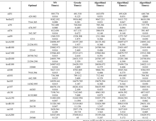
[image:4.595.35.563.132.539.2]In the table below, these three algorithms are compared with NN and Greedy algorithms on library problems [21-23]. The results on the third row shows the best result found when applying NN algorithm starting from each vertices (n times).
Table I. Computational Experiments for Heuristic Algorithms
G Optimal NN Time(s) Greedy Time(s) Algorithm1 Time(s) Algorithm2 Time(s) Algorithm3 Time(s) eil51 429.983 505.774 0.016 481.518 0.125 443.070 0.031 495.628 0.031 440.746 0.000 berlin52 7544.365 8182.192 0.000 9954.062 0.281 9047.211 0.031 9413.732 0.047 8618.198 0.002 st70 678.597 761.689 0.000 746.044 0.485 785.284 0.094 811.974 0.094 727.778 0.011 eil76 545.387 612.656 0.016 617.131 0.672 588.074 0.140 606.117 0.140 581.407 0.010 rat99 1211 1369.535 0.016 1528.308 1.875 1311.904 0.266 1273.747 0.282 1316.432 0.030 kroA100 21236.951 24698.497 0.016 24197.285 1.937 26135.302 0.360 24697.677 0.391 24093.242 0.020 kroB100 22141 25882.973 0.016 25815.214 2.469 24700.544 0.406 23651.697 0.406 23419.490 0.031 kroC100 20750.762 23566.403 0.015 25313.671 2.610 23962.861 0.391 24879.757 0.391 23512.300 0.030 kroD100 21294.290 24855.799 0.016 24631.533 2.359 24783.197 0.422 23201.380 0.390 24758.054 0.010 kroE100 22068 24907.022 0.016 24420.355 2.609 26036.072 0.375 25499.724 0.406 24822.113 0.010 rd100 7910.396 9427.333 0.015 8702.605 2.922 9866.781 0.406 8945.544 0.375 9384.955 0.030 eil101 642.309 736.368 0.015 789.112 2.609 712.461 0.329 694.685 0.359 704.361 0.010 lin105 14382.995 16939.441 0.015 16479.785 3.187 19679.294 0.360 17744.411 0.344 18354.693 0.030 pr107 44303 46678.154 0.016 48261.816 2.109 56635.995 0.453 47060.739 0.438 54003.941 0.010 ch130 6110.860 7198.741 0.016 7142.045 7.688 6963.303 0.875 6636.392 0.953 6873.837 0.055 kroA150 26524 31482.020 0.047 31442.994 11.094 31027.270 1.469 28444.581 1.453 30216.728 0.082 kroB150 26130 31320.340 0.047 31519.083 11.156 31824.589 1.547 30815.938 1.454 29631.101 0.064 rat195 2323 2628.561 0.109 2957.176 29.719 2763.001 3.563 2637.019 3.532 2554.672 0.085 kroA200 29368 34547.691 0.125 37650.812 45 35195.046 5.187 35792.822 5.172 33629.972 0.112
V. NEWHEURISTICALGORITHMS
Once a tour has been generated by some tour construction heuristic, we might wish to improve that solution. There are several ways to do this, but the most common ones are the opt and 3-opt local searches. The 2-opt algorithm basically removes two edges from the tour, and reconnects these two paths which are formed by removing these two edges. There is only one way to reconnect the two paths so that we still have a valid tour (Figure 4, 5). We do this only if the new tour will be shorter. This process of removing and reconnecting the tour continues until no 2-opt improvement is found. The tour we obtain at the end of this process is now 2-optimal. The 3-opt algorithm works in a similar fashion, but instead of removing two edges we remove three. This means that we have two ways of reconnecting the three paths into a valid tour (Figure 6). A 3-opt move can actually be seen as two or three 2-3-opt moves. We finish our search when no more 3-opt moves can improve the tour. If a tour is 3-optimal it is also 2-optimal. If we look at the tour as a permutation of all the cities, a 2-opt
move will result in reversing a segment of the permutation. A 3-opt move can be seen as two or three segment reversals [3].
A. 2-opt and Shifting:
The 2-opt code is as following: for (i = 1;i <= n - 3; i ++)
for (j = i + 2; j <= n - 1; j++) if
(d[a[i]][a[i+1]]+d[a[j]][a[j+1]]>d[a[i]][a[j]] + d[a[i+1]][a[j+1]])
swap(a[i+1], a[j])
vertexes. This whole process is explained in an example below:
Table II. Distance matrix
1 2 3 4 5 6 1 0 1 3 5 3 1
2 1 0 1 3 5 3
3 3 1 0 1 3 5
4 5 3 1 0 1 3
5 3 5 3 1 0 1
6 1 3 5 3 1 0
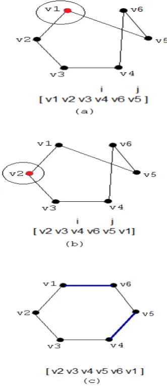
[image:5.595.358.517.126.475.2]For example, let us say that the optimum result of the traveling salesman problem is 6 and the solution vector is [v1v2v3v4v5v6] (6) .The length of the tour of the given tours is computed by giving attention to the distance matrix in Table II. If we apply the 2-opt algorithm to a vector like [v1v2v3v4v6v5](10) whose tour cost is 10, then the algorithm will not make any shifts between the vertexes. Yet, if the elements of solution vector are switched 1 unit to the left, then the 2-opt algorithm will find the optimum result: [v3v4v5v6v1v2](6).
Figure 4. The demonstration of the shifting operation in a 2-opt application on an example
In the same way, if we apply the 2-opt algorithm to the vector, [v1v4v5v2v3v6](18), the algorithm improves this vector three times and the solution vector obtained at the end of the process is [v1v3v2v4v5v6](10). Even if the elements
of this solution vector are shifted 1 unit to the left, there will be no improve. Yet if we apply the 2-opt algorithm after shifting the elements of this solution vector 2 units to the left, then we can obtain the optimum result for the problem [v1v2v3v4v5v6](6).
Figure 5. The demonstration of the double shifting operation in a 2-opt application on an example
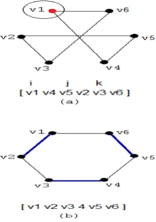
B. 3-opt and Shifting:
The 3-opt code is as following: for(i=1;i<=n-5;i++)
for(j=i+2;j<=n-3;j++)
for(k=j+2;k<=n-1;k++)
if(d[a[i]][a[i+1]]+d[a[j]][a[j+1]] +d[a[k]][a[k+1]]>d[a[i]][a[j+1]] +d[a[j]][a[k+1]]+d[a[k]][a[i+1]])) {
swap(a[i+1], a[j+1]) swap(a[j], a[k]) }
[image:5.595.68.234.308.693.2]Figure 6. The demonstration of the shifting operation in a 3-opt application on an example
C. Compuational Experiments for 3-opt + 2-opt:
In Table III, the second column shows the results of 2-opt and 3-2-opt applications with shifting operation, and the third column shows the results of 2-opt and 3-opt applications without shifting operation. As it can be seen in the table, the results of the applications with shifting operation give better results than the applications without shifting.
Table III. The comparison of the 2-opt and 3-opt applications with and without shifting operation
G 3-opt + 2-opt (S+) 3-opt + 2-opt (S-)
eil51 429.484 456.265
berlin52 7544.365 7993.064
kroA100 21285.443 22146.600
rd100 8101.042 8206.614
lin105 14382.995 14670.207
ch130 6250.213 6409.888
u159 43786.312 45147.919
VI. OTHERIMPROVEDALGORITHMS
Below, a hybrid of NN and greedy algorithms and an improved version of vertex ranking based on learning are presented.
A. Hybrid Heuristic Algorithm:
The algorithm that we propose is a hybrid of the traditional NN and Greedy heuristic algorithm. We start the algorithm with NN for each vertex and repeat it for n times. Each time the algorithm is applied, we give a “priority” to the edge according to the result of the solution. Let the “priority” of the selected edges in the first solution be 1 all the others be 0. Suppose that the length of the first tour is
D
1Then, we add 1 i
D
D
(Here,D
i is the length of the tour, whichis found at step
i
) to the “priorities” of the selected edges. Thus, each edge has a “priority” after n steps. Then, we sort the edges in descending order by “priority” and solve the problem with greedy algorithm. Let the length of the tour be1 n
D
+ , and we add 1 1 nD
D
+ to the “priorities” of the selectededges. At the next steps, the edges are sorted in descending order by their updated “priorities”, and then, we solve the problem with the greedy algorithm. This process continues until there is no change on the sorting anymore. The result of the algorithm is the best solution found during this process. The steps of the algorithm are as follows:
a. Solve the problem n times by NN algorithm starting with different vertices at each time. Find the “priorities” of edges. Assign the best solution, as a record solution.
b. Sort the edges in descending order by “priority”. Then, solve the problem by the greedy algorithm. If the solution is better (smaller) than the record solution update the record.
c. If there is no any change in the sorting then, stops the algorithm otherwise go to Step 2.
B. Hyperheuristic Algorithm (Vertex Ranking):
Finding the initial solution:
For each vertex, find the row sum in the adjacency matrix and assign it to array of sums.
a. For each vertex, find the first shortest edge in the adjacency matrix and increase their importance values an array of importance’s by in this order. b. For each edge, set the priority value in the array of
priorities as the biggest value of its vertices importance values in the array of importance’s. c. Sort the edges decreasingly according to their
importance values. If there are same importance values, sort them decreasingly according to their priority values. If priorities are same too, then sort them increasingly according to their lengths. d. Add the vertex, which will not create a sub tour, to
the solution from the array of importances in order. Improving the initial solution:
e. After finding the initial solution, add 1 to the importance value of the first edge, which is not added to the solution and go to step 4.
If the new solution is worse than the best solution found so far, subtract n from the importance value of the last vertex which is added 1 to its importance value before and add 1 to the importance value of the first edge, which is not added to the solution and go to step 4 again. In other case where the new solution is not worse than the best solution found so far, add 1 to the importance value of the first edge, which is not added to the solution and go to step 4 again. This process is repeated two times. n is the total vertex number of the graph.
The principles of this algorithm can be explained as follows:
[image:6.595.46.271.449.585.2]importance value according to its priority value. Edges are sorted according to their importance values in decreasing order. An initial solution is found using a greedy algorithm in step 5. In step 6, initial solution is tried to improve using a learning based iterative approach.
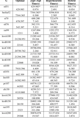
Table IV. Computational experiments for the heuristics, which improve the tour
G Optimal 2opt+3opt Time(s) Hyperheuristic Time(s) Hybrid Time(s) eil51 429.983 429.983* 0.974 444.415 2.491 505.774 0.054 berlin52 7544.365 7544.365* 0.300 8396.818 2.305 8182.192 0.045 st70 678.597 688.280 7.145 722.679 9.043 761.689 0.190 eil76 545.387 562.331 5.211 566.774 13.982 612.655 0.314 rat99 1211 1247.094 3.406 1252.272 62.623 1369.534 0.373 kroA100 21236.951 21285.443 10.264 21936.297 51.252 24698.497 0.536 kroB100 22141 22585.399 5.857 23665.102 52.457 25882.973 0.385 kroC100 20750.762 20786.896 2.264 21954.034 52.911 23566.403 0.398 kroD100 21294.290 21733.785 10.015 23733.511 51.840 24855.799 0.481 kroE100 22068 22331.660 19.028 23102.137 54.109 24907.022 0.398 rd100 7910.396 8101.042 4.409 8544.428 52.012 9427.333 0.385 eil101 642.309 661.138 7.162 678.246 53.687 736.368 0.389 lin105 14382.995 14382.995* 45.414 15730.244 68.545 16939.441 0.724 pr107 44303 44576.123 47.065 44324.838 77.399 46678.154 0.506 ch130 6110.860 6250.213 7.572 6337.452 209.594 7198.741 1.142 kroA150 26524 27229.789 188.898 27968.152 424.945 31482.020 1.401 kroB150 26130 26802.108 264.646 28295.964 408.977 31320.340 1.494 rat195 2323 2473.668 221.204 2472.163 1589.158 2618.045 3.721 kroA200 29368 30876.078 19.547 31137.834 1814.037 34547.691 3.874
C. Computational Experiments for the Heuristics which Improve the Tour:
Table IV shows the result of computational experiments of these 3 algorithms conducted on library problems [21-23]. The best results are marked on the table. As it is shown in the table, best results are usually obtained by “2-opt + 3-opt +shifting”. In Table IV, * sign shows the optimum result.
VII.CONCLUSION
In this study, we have proposed four new heuristics to solve traveling salesman problem. We have offered a number of different NN versions. We have found better solution than NN and greedy by combined them. In addition, we consider the tour-improved techniques; 2opt, 3opt and we have improved their performance by some modification. When we consider the study of old and newly proposed algorithms and the results of computational experiments, it is seen that the best solution is obtained by applying “2opt + 3opt + shifting” on best result found by applying NN algorithm n times, for each vertices as starting vertex. For further study, the
different combinations of the heuristics will be investigated in order to improve the results.
VIII.REFERENCES
[1] D. Applegate, W. Cook, A. Rohe, Chained Lin-Kernighan for Large Traveling Salesman Problems, INFORMS Journal on Computing 15(1) (2003), pp. 82 – 92.
[2] S. Climer, W. Zhang, Rearrangement Clustering: Pitfalls, Remedies, and Applications, Journal of Machine Learning Research 7 (2006), pp. 919 – 943.
[3] G. Gutin, A. Punnen (eds.), The Traveling Salesman Problem and Its Variations, volume 12 of Combinatorial Optimization. Kluwer, Dordrecht, 2002.
[4] M. Held, R. Karp, A Dynamic Programming Approach to Sequencing Problems, Journal of SIAM 10 (1962), pp. 196 – 210.
[5] L. J. Hubert, F. B. Baker, Applications of Combinatorial Programming to Data Analysis: The Traveling Salesman and Related Problems, Psychometrika, 43(1), p. 81-91, 1978.
[6] D. Johnson, C. Papadimitriou, Computational complexity, In Lawler et al, chapter 3, p. 37-86, 1985a.
[7] D. Johnson, C. Papadimitriou (1985b), Performance guarantees for heuristics, In Lawler et al, chapter 5, p. 145-180, 1985.
[8] D.S. Johnson and L.A. McGeoch, The Traveling Salesman Problem: A Case Study, Local Search in Combinatorial Optimization, p. 215-310, John Wiley & Sons, 1997.
[9] O. Johnson, J. Liu, A traveling salesman approach for predicting protein functions, Source Code for Biology and Medicine, 1(3), 1-7, 2006.
[10] A. Land, A. Doig, An Automatic Method for Solving Discrete Programming Problems, Econometrica, 28, p. 497-520, 1960.
[11] E. L. Lawler, J. K. Lenstra, A. H. G. Rinnoy Kan, D. B. Shmoys, The Traveling Salesman Problem: A Guided Tour of Combinatorial Optimization, John Wiley & Sons, 1986.
[12] J. Lenstra, A. R. Kan, Some simple applications of the traveling salesman problem, Operational Research Quarterly, 26(4) (1975), pp. 717-733.
[13] J. K. Lenstra, Clustering a Data Array and the Traveling-Salesman Problem, Operations Research, 22(2) (1974), pp. 413-414.
[14] S. Lin, B. Kernighan, An effective heuristic algorithm for the traveling-salesman problem, Operations Research, 21(2) (1973), pp. 498-516.
[15] F. Nuriyeva, New heuristic algorithms for traveling salesman problem, 25th Conference of European Chapter on Combinatorial Optimization, (ECCO XXV), Antalya, Turkey, April 26 – 28, 2012.
[17] A. Punnen, The Traveling Salesman Problem: Applications, Formulations and Variations, In Gutin and Punnen (2002), chapter 1, pp. 1-28, 2002.
[18] S. S. Ray, S. Bandyopadhyay, S. K. Pal, Gene Ordering in Partitive Clustering using Microarray Expressions, Journal of Biosciences 32(5) (2007), pp. 1019-1025.
[19] C. Rego, F. Glover, Local Search and Metaheuristics, In Gutin and Punnen chapter 8 (2002), pp. 309-368, 2002.
[20] G. Reinelt, The Traveling Salesman: Computational Solutions for TSP Applications, Springer-Verlag, Germany, 1994.
[21]
www.iwr.uni-heidelberg.de/gro
[22] http://comopt.ifi.uni-heidelberg.de/software/TSPLIB95/ST