Volume 3, No. 4, July- August 2012
International Journal of Advanced Research in Computer Science
RESEARCH PAPER
Available Online at www.ijarcs.info
ISSN No. 0976-5697
Reduction of Noise from Speech Signal using Wavelet Thresholding
Deepak Sethi*
Assistant Professor Department of CSE PIET Samalkha
(Panipat) India
Mohit Bansal
Assistant Professor Department of ECE BMIET Sonipat
(Haryana) India
Ashok Saini
Assistant Professor Department of ECE IITM
Murthal India sainiashok2011@gmail.com
Navneet Verma
Assistant Professor Department of CSE PIET Samalkha (Panipat) India
navneet_713@yahoo.com
Abstract: In this paper, an original signal is first superimposed with noise and then the noise is reduced by using wavelet thresholding technique. Signal- to-Noise ratio (SNR) is calculated first on the mix signal (signal superimposed with noise) and then calculate Signal-to-Noise (SNR) after reduction of noise from the mix signal. In this paper, one original signal and two noise signal are used. The wavelets used in this research paper are haar wavelet, Symlets (sym8), Coiflets (coif5), biorthogonal (bior2.2), reverse biorthogonal (rbio2.2) and DMeyer (dmey) wavelet.
Keywords: wavelets, noise reduction, noise types, spectrogram of signal, wavelet thresholding, SNR.
I. INTRODUCTION
In case of audio or speech communication, situation occurs that speech signal is superimposed by background noise. Due to rapid growth in technology, there has been tremendous increase in the level of noise. Noise is added through various devices such as noisy engines, heavy machines, pumps, generators, vehicles etc.
Wavelet denoising algorithm is used for reduction of noise from speech signal. The wavelet denoising technique is called thresholding [1]. Mallat and Hwang [2] have shown that effective noise suppression may be achieved by transforming the noisy signal into the wavelet domain, and preserving only the local maxima of the transform. Alternatively, a reconstruction that uses only the large-magnitude coefficients has been shown to approximate well the uncorrupted signal. In other words, noise suppression is achieved by thresholding the wavelet transform of the contaminated signal. In [3].Donoho employs the thresholding in the wavelet domain and has shown to have near optimal properties for a wide class of signal is corrupted by additive white gaussian noise. The utilization of wavelets in signal and image processing has been found to be a very useful tool for solving various engineering problems, de-noising is one of them. The classical methods based on spectral subtraction [4] are effective for this purpose, however they introduce artificial noise and alter the original signal. Donoho [5] introduced wavelet thresholding (shrinking) as a powerful tool in denoising signals degraded by additive white noise. Although the application of wavelet shrin- king for speech enhancement has been reported in literature there are many problems yet to be resolved for a successful application of the method to speech signals degraded by real environmental noise types. In 1995, wavelet thresholding was firstly introduced by Donoho and Johnstone [6, 7] and was applied to noise reduction
successfully. But its direct application in speech enhancement can not achieve satisfactory results. One of the most problems is that it creates some nonuniform “musical noise” artifacts, also called “liquid noise” [8]. In recent years, a number of attempts have been made to solve this problem [9-12]. Considering that the classical wavelet denoising method thresholds wavelet coefficients point by point, a block thresholding method is proposed in [9] and some improvements are achieved by incorporating intrascale dependencies of neighboring coefficients.
It is a three step procedure. In first step, Discrete Wavelet Transform (DWT) technique is applied to the input signal (noisy signal) to compute the wavelet coefficients. Second step consist of thresholding (soft or hard) these wavelet coefficients and in third step, inverse discrete wavelet transform (IDWT) technique is applied to get the output signal or denoised signal.
Digital Signal Processing, a field which has its roots in
17 th
and 18 th
The purpose of such processing may be to estimate characteristic parameters of a signal or to transform a signal into a form which is in some sense more desirable. Signal processing, in general, has a rich history, and its importance is evident in such diverse fields as biomedical engineering, acoustics, sonar, radar, seismology, speech communication, data communication, nuclear science and many others. In many applications, as, for example, in Electrocardiogram (ECG) analysis or in systems for speech transmission and speech recognition, we may wish to remove interference, such as noise, from the signal or to modify the signal to present it in a form which is more easily interpreted. As another example, a signal transmitted over a communications channel is generally perturbed in a variety of ways, including channel distortion, fading, and the insertion of background noise. One of the objectives at the receiver is to compensate for these disturbances.
century mathematics, has become an important tool in a multitude of diverse fields of science and technology. The field of digital signal processing has grown enormously in the past decade to encompass and provide firm theoretical backgrounds for a large number of individual areas [19]. The term “digital signal processing” may have a different meaning for different people. For example, a binary bit stream can be considered a “digital signal” and the various manipulations, or “signal processing”, performed at the bit level by digital hardware may be construed as “digital signal processing”. But, the viewpoint taken in this thesis is different. Implicit in the definition of digital signal processing (DSP) is the notion of an information-bearing signal that has an analog counterpart. What are manipulated are samples of this implicitly analog signal. Further, these samples are quantized, that is represented using finite precision, with each word representative of the value of the sample of an (implicitly) analog signal. These manipulations, or filters, performed on these samples are arithmetic in nature – additions and multiplications. The definition of DSP includes the processing associated with sampling, conversion between analog and digital domains, and changes in wordlength [20]. Digital Signal Processing is concerned with the representation of signals by sequences of numbers or symbols and the processing of these sequences.
In each case, processing of the signal is required. Signal processing problems are not confined to one-dimensional signals. Many image processing applications require the use of two-dimensional signal processing techniques. This is the case, for example, in x-ray enhancement, the enhancement and analysis of aerial photographs for detection of forest fires or crop damage, the analysis of satellite weather photos, and the enhancement of television transmissions from lunar and deep space probes. Seismic data analysis as required in oil exploration, earthquake measurements and nuclear test monitoring also utilizes multidimensional signal processing techniques [21]. There are many reasons why
digital signal processing of an analog signal may be preferable to processing the signal directly in the analog domain. First, a digital programmable system allows flexibility in reconfiguring the digital signal processing operations simply by changing the program. Reconfiguration of an analog system usually implies a redesign of the hardware followed by testing and verification to see that it operates properly. Accuracy considerations also play an important role in determining the form of the signal processor. Tolerances in analog circuit components make it extremely difficult for the system designer to control the accuracy of an analog signal processing system.
On the other hand, a digital system provides much better control of accuracy requirements. Digital signals are easily stored on magnetic media (tape or disk) without deterioration or loss of signal fidelity beyond that introduced in the A/D conversion. As a consequence, the signals become transportable and can be processed off-line in a remote laboratory. The digital signal processing method also allows for the implementation of more sophisticated signal processing algorithms. It is usually very difficult to perform precise mathematical operations on signals in analog form, but these same operations can be routinely implemented on a digital computer using software. The digital implementation of the signal processing system is almost always cheaper than its analog counterpart as a result of the flexibility for modifications. As a consequence of these advantages, digital signal processing has been applied in practical systems covering a broad range of disciplines. However, digital implementation has its limitations. One practical limitation is the speed of operation of A/D converters and digital signal processors. Signals having extremely wide bandwidths require fast sampling rate A/D converters and fast digital signal processors. Hence there are analog signals with large bandwidths for which a digital processing approach is beyond the state of the art of digital hardware [22] . The techniques and applications of digital signal processing are expanding at a tremendous rate. With the advent of large scale integration and the resulting reduction in cost and size of digital components, together with increasing speed, the class of applications of digital signal processing techniques is growing.
lifting scheme can be used to construct the first-generation wavelet and results in faster, fully in-place implementation of the famous Mallat formula [29, 30]. In [30], Daubechies and Sweldens provided different lifting schemes for a typical wavelet, such as D4, D6, CDF 9–7 and cubic B-spline wavelets. It is easy to see that many wavelet filters (for example, D4, D6 and CDF 9–7 wavelets) are designed with coefficients that are irrational numbers. Infinite precision implementation is thus needed for these filters. In order to achieve wavelet filters with rational coefficients, motivated by the work of Sweldens et al. in [27–30] based on the lifting scheme.
II. NOISE
Noise is a barrier to communication that may weaken or destroy a speech or audio signal. Noise can be classified in number of ways. It can be sub-divided according to source, type, effect or relation to the receiver. According to source, there are two types of noise.
a. external noise b. Internal noise
In case of external noise, noise sources are external to the receiver, and in internal noise, noise created within the receiver itself.
A. Types of Noise:
Some of the very important noises are:
a. Thermal Noise: This noise is generated by thermal agitation of electrons in a conductor. Noise power P is given by:
p= kTDf ……….. (1)
where, k:- Boltzmann’s constant is joules/Kelvin T :- conductor temperature in Kelvin Df:- Bandwidth in Hertz
Thermal noise power remains equal throughout the frequency spectrum. It is also known as Johnson noise.
b. Shot Noise: Shot noise occurs when there is voltage differential. For example, PN junction diode that has voltage differential (potential barrier). Shot noise is produced when electrons and holes cross the barrier, but a resistor does not produce shot noise because there has no potential barrier or voltage differential in between a resistor. When current passes through a resistor, it will not exhibit any fluctuations but when current passes through diode produces small fluctuations. Shot noise depends upon the current passing through the device.
c. 1/f (one-over-f) Noise: It is also known as flicker noise or pink noise. 1/f refers to a time series with random fluctuations.
Power Spectra S(f) is :
S(f) = 1/f b ……….. (2)
Flicker noise is also found in electron flow through a conductor, in environment and also in nuclear radiations [18].
Where, b is very close to 1.
d. Burst noise: Burst noise consists of sudden step-like transitions between two or more levels, as high as several hundre unpredictable times. Each shift in offset voltage or current lasts for several milliseconds, and the intervals between pulses tend to be in the (less than 1
for the popping or crackling sounds it produces in audio circuits.
e. Avalanche noise: Avalanche noise is the noise produced when a junction diode is operated at the onset of voltage gradient develop sufficient energy to dislodge additional carriers through physical impact, creating ragged current flows.
B. Colours of Noise:
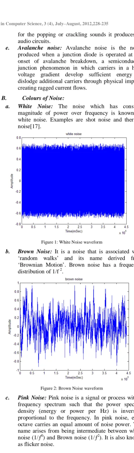
[image:3.595.313.545.0.782.2]a. White Noise: The noise which has constant magnitude of power over frequency is known as white noise. Examples are shot noise and thermal noise[17].
Figure 1: White Noise waveform
[image:3.595.315.544.73.439.2]b. Brown Noise: It is a noise that is associated with ‘random walks’ and its name derived from ‘Brownian Motion’. Brown noise has a frequency distribution of 1/f 2.
Figure 2: Brown Noise waveform
Figure 3: Pink Noise waveform
[image:4.595.323.545.61.399.2]d. Blue Noise: It is just an inverse of pink noise. Intensity is proportional to f.
Figure 4: Blue Noise waveform
e. Violet Noise: Violet noise is just inverse of brown noise, having frequency increase of 6 dB per octave.
Figure 5: Violet Noise waveform
III. WAVELET THRESHOLDING
The wavelet denoising technique is called thresholding. It is divided in three steps as shown in figure 1. The first one consists in computing the coefficients of the wavelet transform (WT) which is a linear operation. The second step consists in thresholding these coefficients. The last step is the inversion of the thresholded coefficients by applying the inverse wavelet transform, which leads to the denoised signal.
A. Types of Thresholding:
[image:4.595.39.283.213.661.2] [image:4.595.331.539.519.748.2]a. Hard Thresholding: Hard Thresholding is the simplest method. Soft Thresholding has nice mathematical properties and the corresponding theoretical results are available. Let t denote the threshold. The hard threshold signal x is x if |x| > t, and 0 if |x|< t [1](figure 11).
b. Soft Thresholding: The soft threshold signal x is sign(x)(|x| - t) if |x| > t, and 0 if |x| < t.(figure 6)
Figure 6: Original Signal, hard thresholding and soft thresholding
Hard thresholding can be described as the usual process of setting to zero the elements whose absolute values are lower than the threshold. Soft thresholding is an extension of hard thresholding, first setting to zero the elements whose absolute values are lower than the threshold, and then shrinking the nonzero coefficients towards 0. The hard procedure creates discontinuities at x = ±t, while the soft procedure does not [1].
IV. ALGORITHM FOR SPEECH SIGNAL
DENOISING
After mixing of noise in original signal, the reduction of noise from signal is done through following steps.
Step 1: The chosen wavelets are haar wavelet, Symlets (sym8), Coiflets (coif5), biorthogonal (bior2.2), reverse biorthogonal (rbio2.2) and DMeyer (dmey) wavelet.
Step 2: Setting the parameters for example soft threshold, threshold selection rule, threshold rescaling, level of decomposition and name of wavelet.
Step 3: Calculate SNR using the formula SNR = PSIGNAL/ PNOISE
V.RESULTS
[image:5.595.326.551.61.266.2]--- (3)
[image:5.595.321.548.67.523.2]Figure 8 shows the waveform of original signal, random noise and mix signal.
[image:5.595.44.272.229.448.2]Figure 8: Waveform of original signal, random noise and mix signal
Figure 9 shows the waveform of original signal, pink noise and mix signal. Figure 10 shows the spectrogram of original signal.
Figure 11 and figure 13 shows the spectrogram of random noise and pink noise. Figure 12 and figure 14 shows the spectrogram of mix signal using random noise and pink noise.
Figure 9: Waveform of original signal, pink noise and mix signal
[image:5.595.326.533.290.505.2]Figure 10: spectrogram of original signal
[image:5.595.326.549.534.754.2]Figure 11: spectrogram of random noise
[image:5.595.49.268.552.769.2]Figure 13: Spectrogram of Pink Noise
Figure 14: Spectrogram of Mix signal using Pink Noise
Figure 15: Waveform of original signal and denoised speech signal using rbio2.2 wavelet
[image:6.595.44.281.278.750.2]Figure 16: Denoised signal spectrogram using rbio2.2 wavelet
Figure 17: Denoised signal spectrogram using coif5 wavelet
After addition of random noise, SNR of mix signal is 7.158
And in case of pink noise SNR is 2.826.
Table 1: Reduction of Noise (Pink Noise) From Signal
Decomposition Level (N) =5
SNR (Signal to Noise Ratio) in dB
Name of Wavelet
Hard Thresholding (dB)
Soft Thresholding (dB)
haar 18.530 18.544
sym8 19.887 20.069
coif5 19.824 20.021
bior2.2 20.458 20.627
rbio2.2 21.089 21.358
[image:6.595.324.555.345.554.2]Table 2: Reduction Of Noise (Random Noise) From Signal
Decomposition Level (N) =5
SNR (Signal to Noise Ratio) in dB
Name of Wavelet Hard Thresholding (dB) Soft Thresholding (dB)
haar 18.661 19.059
sym8 19.591 19.907
coif5 19.442 19.685
bior2.2 20.255 20.499
rbio2.2 21.371 22.213
dmey 19.520 19.648
VI. CONCLUSION
Reverse biorthogonal (rbio2.2) wavelet give better SNR as compare to other wavelets, which means that rbio2.2 is a superior wavelet to reduce noise. Soft thresholding give better SNR as compare to hard thresholding.
The wavelet analysis procedure is to adopt a wavelet prototype function, called "mother wavelet”. Temporal analysis is performed with a contracted, high-frequency version of the prototype wavelet, while frequency analysis is performed with a dilated, low-frequency version of the prototype wavelet. Because the original signal or function can be represented in terms of a wavelet expansion (using coefficients in a linear combination of the wavelet functions), data operations can be performed using just the corresponding wavelet coefficients. And if you further choose the best wavelets adapted to your data, or truncate the coefficients below a threshold, your data is sparsely represented. This "sparse coding" makes wavelets an excellent tool in the field of data compression. Other applied fields that are making use of wavelets are: astronomy, acoustics, nuclear engineering, sub-band coding, signal and image processing, neurophysiology, music, magnetic resonance imaging, speech discrimination, optics, fractals, turbulence, earthquake-prediction, radar, human vision, and pure mathematics applications such as solving partial differential equations[31].
VII. REFERENCES
[1]. Mahesh S. Chavan, Nikos Mastorakis, “Studies on
Implementation of Harr and daubechies Wavelet for Denoising of Speech Signal” INTERNATIONAL JOURNAL OF CIRCUITS, SYSTEMS AND SIGNAL PROCESSING Issue 3, Volume 4, 2010.
[2]. S. Mallat and W. L. Hwang, “Singularity detection and processing with wavelets” IEEE Trans.on Infomation Theory, vol. IT-38, pp. 617-643, 1992.
[3]. D, Donoho and I. Johnstone, “Adapting to unknown
smoothness via wavelet shrinkage,” USA,vol. 90, pp. 1200-1223, 1995.
[4]. S.F. Boll, “Suppression of acoustic noise inspeech using spectral subtraction”. IEEE Trans. Acoust. Speech. Signal process., vol. 27, pp. 113-120, April 1979.
[5]. D.L.Donoho, “De-noising by soft-thresholding”, IEEE Trans.on Inf. Theory, 41,3, pp.613-627, 1995.
[6]. D.L. Donoho and I.M. Johnstone, “Ideal spatial adaption via wavelet shrinkage,” Bionetrika, vol. 81, no. 3, 1994, pp. 425-455.
[7]. D.L. Donoho and I.M. Johnstone, “Adapting to unknown smoothness via wavelet shrinkage,” J. Amer. Statist. Assoc., vol. 90, no. 432, 1995,pp. 1200-1224.
[8]. H. Sheikhzadeh and H. R. Abutalebi, “An improved
wavelet-based speech enhancment system,” in Proc. Of Eurospeech, 2001, pp. 1855-1858.
[9]. T. Cai and B. W. Silverman, “Incorporate information on neighbouring coefficients into wavelet estimation,” Sankhya, vol. 63, 2001, pp. 127-148.
[10]. M. Bahoura and J. Rouat, “Wavelet speech enhancement based on timescale adaptation,” Speech Commun., vol. 48, no. 12, 2006, pp.1620-1637.
[11]. M. T. Johnson, X. Yuan and Y. Ren, “Speech signal enhancement through adaptive wavelet thresholding,” Speech Commun., vol. 49, 2007,pp. 123-133.
[12]. Y. Ren and M. T. Johnson, “Auditory coding based speech enhancement,” in Proc. IEEE Int. Conf. Acoustic, Speech, Signal Processing (ICASSP), 2009, pp. 4685-4688.
[13]. Seong Rag Kim, Adam Efron. “Adaptive Robust Impulse Noise Filtering,” IEEE Trans. Signal Processing, 1995, 43(8), pp.1855~1866.
[14]. S. Zhang and M.A. Karim. “A new impulse detector for switching median filters,” IEEE Signal Process. Lett., vol. 9, no. 11, 2002, pp.360-363.
[15]. C. Chandra, M. S. Moore, S. K. Mitra, “An efficient method for the removal of impulse noise from speech and audio signals,” Proceedings of ISCAS 1998, vol. 4, pp.206-208, Jun 1998.
[16]. R. C. Nongpiur. ‘‘Impulse Noise Removal In Speech Using Wavelets,’’. IEEE ICASSP, 2008, pp.1593~1596.
[17].
[18]. http://en.wikipedia.org/wiki/1/f_noise
[19]. Alan V. Oppenheim and Ronald W. Schafer, Digital Signal Processing. Prentice-Hall, Inc., Englewood Cliffs, N.J., U.S.A, 2001.
[20]. Kishan Shenoi, Digital Signal Processing in
Telecommunications. Prentice-Hall PTR, NJ, 1995.
[21]. Lawrence R. Rabiner and Bernard Gold, Theory and Application of Digital Signal Processing. Prentice-Hall, Inc. Englewood Cliffs, New Jersey, 1995.
[22]. J. Proakis, Charles M. Rader, Fuyun Ling, Christopher L. Nikias, Advanced Digital Signal Processing. MacMillan Coll Div, 1992.
[23]. Mallat, S.G.: ‘Multiresolution approximation and wavelet orthogonal base of L2
[24]. Daubechies, I.: ‘Orthonormal bases of compactly supported wavelets’, Commun. Pure Appl. Maths., 1988, 41, (2), pp. 909–980
(R)’, Trans. Am. Math. Soc., 1989, 315, (1), pp. 68–88
[25]. Cohen, A., Daubechies, I., and Feauveau, J.C.:
[26]. Vetterli, M., and Herley, C.: ‘Wavelets and filters: theory and design’, IEEE Trans. Signal Process., 1992, 40, (12), pp. 2207–2232
[27]. Sweldens, W.: ‘The lifting scheme: a new philosophy in biorthogonal wavelet constructions’, Proc. SPIE-Int. Soc. Opt. Eng., 1995, 2569, pp. 68–79
[28]. Sweldens, W.: ‘The lifting scheme: a custom-design construction of biorthogonal wavelets’, Appl. Comput. Harmon. Anal., 1996, 3, (2), pp. 186–200
[29]. Sweldens, W.: ‘The lifting scheme: a construction of second generation wavelets’, SIAM J. Math. Anal., 1997, 29, (2), pp. 511–546
[30]. Daubechies, I., and Sweldens, W.: ‘Factoring wavelet transforms into lifting step’, J. Fourier Anal. Appl., 1998, 4, (3), pp. 247–269.