Page 1 of 11 Big-data Clinical Trial Column
Balance diagnostics after propensity score matching
Zhongheng Zhang1, Hwa Jung Kim2,3, Guillaume Lonjon4,5,6,7, Yibing Zhu8; written on behalf of AME Big-Data Clinical Trial Collaborative Group
1Department of Emergency Medicine, Sir Run Run Shaw Hospital, Zhejiang University School of Medicine, Hangzhou 310016, China; 2Department of Clinical Epidemiology and Biostatistics, Asan Medical Center, Seoul, Korea; 3Department of Preventive Medicine, University of Ulsan College of Medicine, Seoul, Korea; 4INSERM, UMR 1153, Centre of Research in Epidemiology and Statistics Sorbonne Paris Cite´ (CRESS), METHODS Team, Paris, France; 5Orthopaedic Department, Assistance Publique-Hoˆpitaux de Paris, Paris, France; 6Hospital Georges Pompidou, Paris, France; 7Medical School, Paris Descartes University, Sorbonne Paris Cité, Paris, France; 8ICU, Fuxing Hospital, Capital Medical University, Beijing 100045, China
Correspondence to: Zhongheng Zhang. No. 3, East Qingchun Road, Hangzhou 310016, China. Email: [email protected].
Abstract: Propensity score matching (PSM) is a popular method in clinical researches to create a balanced covariate distribution between treated and untreated groups. However, the balance diagnostics are often not appropriately conducted and reported in the literature and therefore the validity of the findings from the PSM analysis is not warranted. The special article aims to outline the methods used for assessing balance in covariates after PSM. Standardized mean difference (SMD) is the most commonly used statistic to examine the balance of covariate distribution between treatment groups. Because SMD is independent of the unit of measurement, it allows comparison between variables with different unit of measurement. SMD can be reported with plot. Variance is the second central moment and should also be compared in the matched sample. Finally, a correct specification of the propensity score model (e.g., linearity and additivity) should be re-assessed if there is evidence of imbalance between treated and untreated. R code for the implementation of balance diagnostics is provided and explained.
Keywords: Propensity score; standardized mean difference (SMD); balance diagnostics; prognostic score
Submitted Oct 29, 2018. Accepted for publication Dec 05, 2018. doi: 10.21037/atm.2018.12.10
View this article at: http://dx.doi.org/10.21037/atm.2018.12.10
Introduction
Propensity score analysis has been widely used in medical literature. Propensity score is the probability of treatment assignment conditional on the baseline covariates. Conditional on propensity score, the baseline covariates are expected to be balanced between treated and untreated groups. However, the imbalances of baseline characteristics between two or more treatment groups can still exist if the statistical model used to calculate the propensity score is mis-specified. Thus, it is of vital importance to appropriately carry out balance diagnostics after propensity score matching (PSM) and report the results of the diagnostic analysis. It has been showed that the reporting quality of observational studies using PSM was suboptimal (1-4). Among others, one of the key areas to be improved
working example for the illustration purpose; (II) PSM for the simulated dataset; (III) standardized mean difference (SMD) for assessing covariate balance after matching; (IV) other quantities such as variance ratio and prognostic score to assess covariate balance; and (V) possible solutions to re-specification of the propensity score model when there is evidence of imbalance.
Working example
A simulated dataset is used for the illustration purpose. First, we create a function named psSim(), which simulates a dataset with covariates, treatment group and mortality outcome.
> psSim<-function(CatVarN=2,ContVarN=2, seed=123,n=1000){
set.seed(seed);
Xcont <- replicate(ContVarN, rnorm(n))
Xcat <- replicate(CatVarN, rbinom(n,size = 1,prob = 0.3)) linpredT<-cbind(1, Xcont,Xcat) %*%
sample(c(-5:-1,1:5), 1+CatVarN+ContVarN) + rnorm(n,-0.8,1)
probTreatment <- exp(linpredT) / (1 + exp(linpredT)) Treat <- rbinom(n, 1, probTreatment);
linpredY <- 1 + cbind(Xcont,Xcat) %*% rep(1, CatVarN+ContVarN) +
Treat + rnorm(n, -2, 2); prY = 1/(1+exp(-linpredY)); mort <- rbinom(n,1,prY);
dt <- data.frame(Xcont=Xcont,Xcat=Xcat,Treat, mort) return(dt)
}
dt<-psSim();
> str(dt)
'data.frame': 1000 obs. of 6 variables:
$ Xcont.1: num -0.5605 -0.2302 1.5587 0.0705 0.1293 ... $ Xcont.2: num -0.996 -1.04 -0.018 -0.132 -2.549 ... $ Xcat.1 : int 0 1 0 1 0 0 1 0 0 1 ...
$ Xcat.2 : int 0 1 1 0 0 0 0 0 1 0 ... $ Treat : int 1 1 0 1 1 0 0 0 0 1 ... $ mort : int 0 1 0 0 0 1 1 1 0 0 ...
The returned object of the psSim() function is a data frame containing 6 variables. Xcont.1 and Xcont.2 are
numeric variables; and Xcat.1 and Xcat.2 are categorical variables with levels 0 and 1. Note that only 4 variables are generated, but there can be much more baseline variables in real practice. Treat represents the assignment of treatment groups. mort is the vital status denoted as 1 for dead and 0 for alive.
Next, we examine the balance of covariates between treated and untreated groups. The tableone package (v0.9.3) will be used to compare baseline characteristics between the two groups.
> library(tableone) > myVars <- names(dt)[1:4]
> tabbefore <- CreateTableOne(vars = myVars, data = dt,
strata = 'Treat',
factorVars = c('Xcat.1','Xcat.2'), smd = T)
> tabbefore <- print(tabbefore, printToggle = FALSE,
noSpaces = TRUE, smd=TRUE, quote=T)
> tabbefore; Stratified by Treat
0 1 p test SMD
n 682 318
Xcont.1 (mean (sd)) 0.25 (0.94) -0.49 (0.91) <0.001 0.800
Xcont.2 (mean (sd)) 0.40 (0.88) -0.72 (0.83) <0.001 1.312
Xcat.1 = 1 (%) 132 (19.4) 150 (47.2) <0.001 0.618
Xcat.2 = 1 (%) 271 (39.7) 31 (9.7) <0.001 0.741
The results show that there are significant differences in variables Xcont.1, Xcont.2, Xcat.1 and Xcat.2 with SMD greater than 0.1, a threshold being recommended for declaring imbalance (7). SMD is given by the following equation (8):
1 2 2 2 2
1 2 / 2
X X
SMD
S S
− =
+
( )
where X1 and X2 are sample mean for the treated and
control groups, respectively; 2 1
S and 2 2
S are sample variance for the treated and control groups. It is noted that the difference between two groups is no long dependent on the unit of measurement and thus variables with different types of measurements can be compared on SMD scale.
1 11 22 2 [ (1 ) (1 )] / 2
p p SMD
p p p p
− =
− + −
where p1 and p2 are prevalence of dichotomous variables in
the treated and control groups, respectively. Again, a SMD greater than 0.1 can be considered as a sign of imbalance.
PSM
PSM can be easily done with the MatchIt package (v3.0.2).
> library(MatchIt);
> m.out<-matchit(Treat~ Xcont.1+Xcont.2+Xcat.1+Xcat.2, dt, method = "nearest", caliper=0.1)
In the example, all covariates are used to predict the treatment group. The nearest neighbor (NN) matching algorithm goes through the potential matches in the untreated samples and selects the closest unmatched subject in terms of propensity score to match the treated subject (9). However, the NN matching is at risk of bad matches when the closest neighbor is far away. The caliper imposes a tolerance level on the maximum PS distance. Only NNs within the caliper size can be matched. The caliper argument in the matchit() function can be used to define a caliper.
SMD
SMD is probably the most widely used statistic for the assessment of balance after PSM, because it is easy to compute and understand. The cobalt package (v3.4.1) is excellent in calculating SMD and other useful quantities.
> bal.tab(m.out,m.threshold=0.1) Call
matchit(formula = Treat ~ Xcont.1 + Xcont.2 + Xcat.1 + Xcat.2, data = dt, method = "nearest",
caliper = 0.1)
Balance measures
Type Diff.Adj M.Threshold
distance Distance 0.0746
Xcont.1 Contin. -0.0745 Balanced, <0.1
Xcont.2 Contin. 0.0591 Balanced, <0.1
Xcat.1 Binary 0.0326 Balanced, <0.1
Xcat.2 Binary -0.0326 Balanced, <0.1
Balance tally for mean differences
count
Balanced, <0.1 4
Not Balanced, >0.1 0
Variable with the greatest mean difference
Variable Diff.Adj M.Threshold
X1 -0.0745 Balanced, <0.1
Sample sizes
Control Treated
All 682 318
Matched 92 92
Unmatched 590 226
The above output shows that when setting the threshold for mean difference to 0.1, all covariates were balanced after PSM. The (standardized) difference in means between the two groups after matching is shown in the third column of the first table. Note that the distance measure generated by matchit() is automatically included. By default, the bal.tab() function calculates the raw difference in proportions for binary covariates (X1.1 and X2.1), instead of the SMD. The following two tables show the summary statistics for the matching results. The last table shows number of subjects before and after matching in the control and treated groups.
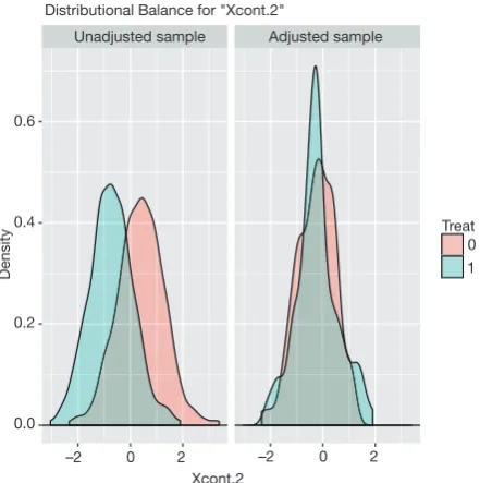
The distribution of continuous and categorical variables stratified by treatment group before and after matching can be visualized with the bal.plot() function.
> bal.plot(m.out,var.name = 'Xcont.2',which = 'both') > bal.plot(m.out,var.name = 'Xcat.1',which = 'both')
Publication quality plot
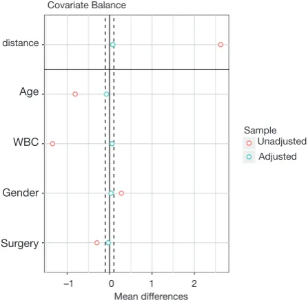
Covariate balance for all variables can be displayed in a so-called Love plot. Furthermore, the variable name can be modified to meet the publication standard.
> v <- data.frame(old = c("Xcont.1","Xcont.2","Xcat.1","Xcat.2"), new = c("Age", "WBC", "Gender",'Surgery'))
> love.plot(bal.tab(m.out, m.threshold=0.1), stat = "mean.diffs", var.names = v, abs = F)
Variable names such as Xcat.1 and Xcont.2 are not meaningful for subject-matter audience, thus we change the names to “Age”, “WBC”, “Gender” and “Surgery”. Figure 3 shows the mean difference in all variables between treated and control groups before and after PSM. Two dashed vertical lines indicate the threshold within which the balance is considered to be achieved.
Statistical inference to compare difference after PSM
Sometimes, investigators may want to compare difference between treated and control groups after PSM. The tableone package (v0.9.3) can do the work and produce high quality tables.
> df.match <- match.data(m.out)[1:ncol(dt)] > tabafter <- CreateTableOne(vars = myVars, data = df.match,
strata = 'Treat',
factorVars = c('Xcat.1','Xcat.2'), smd = T)
> tabafter <- print(tabafter, printToggle = FALSE, noSpaces = TRUE,smd=TRUE) > tabafter;
Stratified by Treat
0 1 p test SMD
n 92 92
Xcont.1 (mean (sd)) -0.12 (0.83) -0.19 (0.84) 0.584 0.081
Xcont.2 (mean (sd)) -0.27 (0.72) -0.22 (0.80) 0.662 0.064
Xcat.1 = 1 (%) 33 (35.9) 36 (39.1) 0.761 0.067
Xcat.2 = 1 (%) 19 (20.7) 16 (17.4) 0.707 0.083
Also note that the mean difference obtained by CreateTableOne() function is different from that obtained by bal.tab() function. In fact, The computed spread (variance) bal.tab() uses is always that of the full, unadjusted sample (i.e., before matching), while the CreateTableOne() computes spread using the matched sample. The rationale for the use of the standard deviation of the unmatched
Distributional Balance for "Xcont.2"
Unadjusted sample Adjusted sample
Treat 0 1
Xcont.2
–2 0 2 –2 0 2
Density
0.6
0.4
0.2
[image:4.595.57.278.84.306.2]0.0
Figure 1 Density function showing the distribution balance for variable Xcont.2 before and after PSM. PSM, propensity score matching.
Distributional Balance for "Xcat.1"
Unadjusted sample Adjusted sample
Pr
oportion
Xcat.1
Treat 0 1 0.8
0.6
0.4
0.2
0.0
0 1 0 1
sample is that it prevents the paradoxical situation that occurs when PSM decreases both the spread of the sample and the mean difference, yielding a larger SMD than that prior to adjustment, even though the matched groups are now more similar. By using the same standard deviation before and after matching, the change in balance is independent of the change in mean difference, rather than being conflated with an accompanying change in standard deviation (10). Furthermore, while the CreateTableOne() reports SMD for categorical variables, bal.tab() reports absolute difference for the categorical variables.
Below we show the calculation of SMD in both functions by using Xcont.1 as an example. SMD is computed by using standard deviation of the matched sample, as that computed in CreateTableOne():
> abs((mean(df.match[df.match$Treat==1,'Xcont.1'])-mean(df.match[df.match$Treat==0,'Xcont.1'])))/ sqrt((var(df.match[df.match$Treat==1,'Xcont.1'])+ var(df.match[df.match$Treat==0,'Xcont.1']))/2) [1] 0.08097716
SMD is computed using standard deviation of the treated group in the unmatched sample, as that computed in bal. tab():
> (mean(df.match[df.match$Treat==1,'Xcont.1'])-mean(df.match[df.match$Treat==0,'Xcont.1']))/ sqrt((var(dt[dt$Treat==1,'Xcont.1'])))
[1] -0.07446378
Although significance testing is commonly used to assessing balance in observational studies, it is inappropriate for the following reasons. The sample size of the study population after PSM is reduced, and thus the power to detect statistical significance is also reduced. Non-significance after PSM may simply due to the reduced sample size rather than improved balance. In other words, the statistical insignificance can occur when we randomly drop more number of controls (11). Also, it should be pointed out that evaluating imbalance using hypothesis testing and the corresponding p-value should be used with caution, as spurious statistically significant difference can be detected due to multiple testing on the covariates even when there is no true difference between the distribution of these covariates.
Variance ratio
Variance is the second central moment about the mean of a random variable. It reflects one aspect of the property of a probability distribution. An ideal balance after PSM is that all central moments are the same between the treated and untreated groups. For continuous variables, the variance should also be compared in the matched sample (12). Variance ratio can be displayed with the bal. tab() function. A variance ratio of 1 in matched sample indicates a good matching, and a variance ratio below 2 is generally acceptable.
> bal.tab(m.out,v.threshold=2) Call
matchit(formula = Treat ~ Xcont.1 + Xcont.2 + Xcat.1 + Xcat.2, data = dt, method = "nearest",
caliper = 0.1)
Balance measures
Type Diff.Adj V.Ratio.Adj V.Threshold
distance Distance 0.0746 1.0765
Xcont.1 Contin. -0.0745 1.0115 Balanced, <2
Sample Unadjusted Adjusted
Mean differences Covariate Balance
distance
Age
WBC
Gender
Surgery
[image:5.595.54.278.85.303.2]–1 0 1 2
Xcont.2 Contin. 0.0591 1.2468 Balanced, <2
Xcat.1 Binary 0.0326
Xcat.2 Binary -0.0326
Balance tally for variance ratios
count Balanced, <2 2 Not Balanced, >2 0
Variable with the greatest variance ratio
Variable V.Ratio.Adj V.Threshold
X2 1.2468 Balanced, <2
Sample sizes
Control Treated
All 682 318
Matched 92 92
Unmatched 590 226
Prognostic score for assessing balance
The prognostic score is defined as the predicted probability of outcome under the control condition. It can be estimated by regressing the outcome on covariates in the control group. Then that fitted model is used to predict outcome for all subjects (13). Simulation study has demonstrated that the prognostic score greatly outperforms mean differences on covariates and significance tests in assessing balance (7). Prognostic scores most highly correlate with bias among all balance measures such as SMD in covariates and t-statistic. There are typically three steps involving balance diagnostics using prognostic score: (I) fit an outcome model in the control group; (II) estimate model-based outcome for both treated and untreated subjects; and (III) compare the SMD of the prognostic scores in the treated and control groups.
> ctrl.data <- dt[dt$Treat == 0,]
> ctrl.fit <- glm(mort ~ Xcont.1+Xcont.2+Xcat.1+Xcat.2, data = ctrl.data)
> dt$prog.score <- predict(ctrl.fit, dt) > bal.tab(m.out, distance = dt["prog.score"]) Call
matchit(formula = Treat ~ Xcont.1 + Xcont.2 + Xcat.1 + Xcat.2, data = dt, method = "nearest", caliper = 0.1)
Balance measures
Type Diff.Adj
prog.score Distance -0.0007
distance Distance 0.0746
Xcont.1 Contin. -0.0745
Xcont.2 Contin. 0.0591
Xcat.1 Binary 0.0326
Xcat.2 Binary -0.0326
Sample sizes
Control Treated
All 682 318
Matched 92 92
Unmatched 590 226
It is noted from the above output that the SMD of the prognostic scores is −0.0007, which indicates a balanced sample.
Methods to identify evidence of model misspecification
If there is evidence of imbalance between treated and control groups (i.e., SMD >0.1) after PSM, investigators may need to check for the mis-specification of the PS model. There are several conditions that must be fulfilled before fitting a logistic regression model such as linearity and additivity.
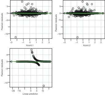
Linearity assumption can be checked by plotting residual against each individual numeric variable.
> library(car)
> mod1<-glm(Treat~Xcont.1+Xcont.2+Xcat.1+Xcat.2, dt,family = binomial)
> residualPlots(mod1,terms=~Xcont.1+Xcont.2,fitted=T)
Test stat Pr(>|t|)
Xcont.1 0.474 0.491
Xcont.2 1.094 0.296
then refit the model used for the estimation of propensity score. The residualPlots() function generates plot for assessing linearity (Figure 4). The linearity assumption is fulfilled when the points on the plot are randomly scattered around zero, so assuming that the error terms have a mean of zero is reasonable. The vertical width of the scatter doesn’t appear to increase or decrease across the fitted values. If the smoothed curve of the scatter points takes a curved pattern, some higher orders terms or cubic spline function can be added for the specific variable in fitting the propensity score model. Assessing linearity is just an example to improve the propensity score model, Austin [2011] indicated that: “one can modify the propensity score by including additional covariates, by adding interactions between covariates that are already in the model, or by modeling the relationship between continuous covariates and treatment status using nonlinear terms.” (14). Furthermore, machine learning algorithms such as classification and regression trees (CART), random forest and neural networks can be employed to improve the specification of the propensity score model (15). These methods account for interaction
and non-linearity without the need to explicitly specify them. Simulated study demonstrated that these advanced methods can help to improve balance between treated and untreated groups (16).
Summary
[image:7.595.124.467.88.397.2]The paper reviewed several methods to assess covariate balance after PSM. SMD is the most widely used quantity and is more comprehensible for subject-matter audience. Statistical inference is also used in the literature, but it is flawed that statistical insignificance after PSM is only a reflection of reduced sample size. Variance is the second central moment about the mean of a random variable. Since the treated and control groups are assumed to be from the sample population after PSM, the variances of the two should be the same. Thus, a variance ratio approaching 1 is the evidence of balance. Prognostic score is the predicted probability of outcome under the control condition, and SMD of prognostic score is found to be a good quantity in assessing balance.
Figure 4 Residual plot to examine non-linearity for continuous variables.
Xcont.1
Pearson r
esiduals
–3 –1 0 1 2 3
–15 5
0
5
0
5
0
Pearson r
esiduals
Xcont.2
–3 –1 0 1 2 3
–15
Pearson r
esiduals
Linear predictor –15
–20 –10 0 5 10 –5
–5
Acknowledgements
We would like to thank Noah Greifer for his valuable comments to improve the manuscript.
Footnote
Conflicts of Interest: The authors have no conflicts of interest to declare.
References
1. Austin PC. Primer on statistical interpretation or methods report card on propensity-score matching in the cardiology literature from 2004 to 2006: a systematic review. Circ Cardiovasc Qual Outcomes 2008;1:62-7.
2. Austin PC. A critical appraisal of propensity-score
matching in the medical literature between 1996 and 2003. Stat Med 2008;27:2037-49.
3. Gayat E, Pirracchio R, Resche-Rigon M, et al. Propensity scores in intensive care and anaesthesiology literature: a systematic review. Intensive Care Med 2010;36:1993-2003. 4. Lonjon G, Porcher R, Ergina P, et al. Potential Pitfalls
of Reporting and Bias in Observational Studies With Propensity Score Analysis Assessing a Surgical Procedure: A Methodological Systematic Review. Ann Surg
2017;265:901-9.
5. Zakrison TL, Austin PC, McCredie VA. A systematic review of propensity score methods in the acute care surgery literature: avoiding the pitfalls and proposing a set of reporting guidelines. Eur J Trauma Emerg Surg 2018;44:385-95.
6. Austin PC. Balance diagnostics for comparing the
distribution of baseline covariates between treatment groups in propensity-score matched samples. Stat Med 2009;28:3083-107.
7. Stuart EA, Lee BK, Leacy FP. Prognostic score-based balance measures can be a useful diagnostic for propensity score methods in comparative effectiveness research. J Clin Epidemiol 2013;66:S84-S90.e1.
8. Flury BK, Riedwyl H. Standard distance in univariate and multivariate analysis. American Statistician 1986;40:249-51.
9. Austin PC. A comparison of 12 algorithms for matching on the propensity score. Stat Med 2014;33:1057-69. 10. Stuart EA. Matching methods for causal inference: A
review and a look forward. Stat Sci 2010;25:1-21. 11. Imai K, King G, Stuart EA. Misunderstandings between
experimentalists and observationalists about causal inference. J R Statist Soc A 2008;171:481-502. 12. Ho DE, Imai K, King G, et al. Matching as
Nonparametric Preprocessing for Reducing Model Dependence in Parametric Causal Inference. Political Analysis 2017;15:199-236.
13. Hansen BB. The prognostic analogue of the propensity score. Biometrika 2008;95:481-8.
14. Austin PC. An introduction to propensity score methods for reducing the effects of confounding in observational studies. Multivariate Behav Res 2011;46:399-424. 15. Westreich D, Lessler J, Funk MJ. Propensity score
estimation: neural networks, support vector machines,
decision trees (CART), and meta-classifiers as alternatives
to logistic regression. J Clin Epidemiol 2010;63:826-33. 16. Lee BK, Lessler J, Stuart EA. Improving propensity
score weighting using machine learning. Stat Med 2010;29:337-46.