Particle Swarm Optimization Based Tuning of PID Controller for Robot Arm Joint Control

(1)

Particle Swarm Optimization Based Tuning of

PID Controller for Robot Arm Joint Control

V. Naga Babu1, A. Srisailaja2

Assistant Professor, Dept. of EEE, Gudlavalleru Engineering College, Gudlavalleru, AP, India1

PG Student [Control Systems], Dept. of EEE, Gudlavalleru Engineering College, Gudlavalleru, AP, India2

ABSTRACT: Most fuzzy controllers have been treated and utilized as ebony-box controllers in the sense that their analytical structures are unknown. Kenning the explicit structure information will enable one to insightfully understand how a fuzzy control works. In this paper analytical structure of fuzzy PID controller is developed with minimum number of regions and rules compared to already subsisting methods. The efficacy of the controller is tested on Robot arm. Results are compared with the conventional controller.

KEYWORDS: Fuzzy controller, Robot arm. Triangular fuzzy sets.

I.INTRODUCTION

Fuzzy controllers are constructed via soi-disant perspicacious system approaches as opposed to the mathematical approaches exclusively utilized in conventional control. The fuzzy controllers have been treated and utilized as ebony box controllers. Without analytical structure information, precise and efficacious mathematical analysis and design are very arduous to achieve. Availability of the structure information may lead to less trail and error effort and engender better control performance.

The fuzzy AND operators that are widely used are Product AND operator and Zadeh AND operator. Deriving analytical structure of the fuzzy controller that utilizes the former operator is not arduous, regardless of the shape of the input fuzzy sets. This is because it is straightforward to carry out multiplication of multiple membership functions in a fuzzy rule. However, revealing the analytical structure of a fuzzy controller that utilizes Zadeh AND operator is far more arduous even for triangular input fuzzy sets, which are simplest fuzzy sets because this operator requires the comparison of membership functions. In 1990 a technique in the literature to cover Zadeh AND operator and a particular class of symmetric trapezoidal fuzzy sets [1] is developed. That method is widely used (e.g. [2], [3] and [4]). Later it is generalized to cover arbitrary trapezoidal fuzzy sets [5]. Then a technique of deriving input output structure applicable to arbitrary types of input fuzzy sets is withal developed [6]. Recently that is elongated to derive the relationship between input space divisions needed due to the utilization of Zadeh AND operator and input fuzzy sets [7] [8] [9].The incrementing demand on robotic system performance leads to the utilization of advanced control strategies. It has been reported that authentic-time control of a manipulator predicated on a detailed mathematical model is arduous to achieve, as the model is both involute and nonlinear. In such situations fuzzy controllers do well. In this paper the robotic arm control is simulated to ken the efficacy of the fuzzy controller utilizing symmetrical input membership functions.

II. DEVELOPMENT OF A GENERAL TECHNIQUE

(2)

Fig 1: The structure of FPID Controller

With these three inputs the structure of the FLC is compared of two independent parallel fuzzy control blocks, each of which contains the corresponding fuzzy control rules and a defuzzifier. The incremental output of the FLC is composed by algebraically integrating the outputs of the two fuzzy control blocks. The following notations are employed.

e(t)= set point-y(t), e(nT) = sample [e(t)] e~(nT) = F(e*), e*=GE e(nT)

r(nT) = [e(nT)-e(nT-T)]/T r~(nT) = F(r*), r* = GR r(nT) a(nT) = [r(nT)-r(nT-T)]/T

= [e(nT)-2e(nT-T)+e(nT-2T)]/T2 a~(nT) = F(a*), a* = GA a(nT) u(nT) = du(nT)+u(nT-T) du(nT) = GU dU(nT) dU(nT) = dU1(nT)+dU2(nT)

Where n is positive integer and T is the sampling period. y(nT), e(nT), r(nT) and a(nT) denote process output, error, rate and acc at sampling time nT, respectively. GE (gain for error) is the input scalar for rate, GA (gain for acc) the input scalar for acc and GU (gain for controller output) the output scalar of the FLC. F(.) describes the fuzzification of the scaled output of the FLC at sampling time nT.dUi(nT) (i=1,2) designate the incremental output of the fuzzy control block i from the defuzzification of the fuzzy set ‘output i’ ui~(nT) at sampling time nT. Thus the FLC includes the following components.

(1) Input scalars GE, GR, GA and output scalar GU

(2) Fuzzification algorithms for scaled error e*, scaled rate r*, scaled acc a* and output of each control block. (3) Fuzzy control rules for each control block.

(4) Fuzzy decision-making logic to evaluate the fuzzy control rules for each control block.

(5) A defuzzification algorithm to obtain the crisp output of each control block for the control of process.

(3)

Fig. 3 Output of fuzzy control block 1 and 2

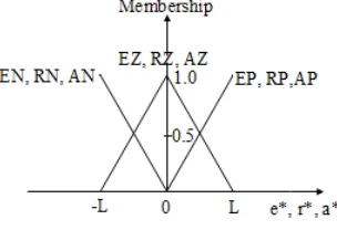
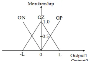
A. Fuzzification Algorithms: The fuzzification for scaled inputs is shown in Fig. 2. The fuzzy set ‘error’ has three membership EP(error positive), EZ(error zero) and EN(error negative), the fuzzy set ‘rate’ has three members RP(rate positive), RZ(rate zero) and RN(rate negative), the fuzzy set ‘acc’ also has three members AP(acc positive), AZ(acc zero) and AN(acc negative). The fuzzy set ‘output1 and output2’ has three members OP(output positive), OZ(output zero) and ON(output negative) as shown in Fig.3.

B. Fuzzy Control Rules

For the fuzzy control rules for each fuzzy control block 1, nine control rules are given as: (R1)1 : IF error = EN and rate = RN THEN output = ON, h-2

(R2)1 : IF error = EZ and rate = RN THEN output = ON, h-1

(R3)1 : IF error = EP and rate = RN THEN output = OZ, h0

(R4)1 : IF error = EN and rate = RZ THEN output = ON, h-1

(R5)1 : IF error = EZ and rate = RZ THEN output = OZ, h0

(R6)1 : IF error = EP and rate = RZ THEN output = OP, h1

(R7)1 : IF error = EN and rate = RP THEN output = OZ, h0

(R8)1 : IF error = EZ and rate = RP THEN output = OP, h1

(R9)1 : IF error = EP and rate = RP THEN output = OP, h2

For the fuzzy control block 2, nine control rules, are given as: (R1)2 : IF rate = RN and acc = AN THEN output = ON, h-2

(R2)2 : IF rate = RZ and acc = AN THEN output = ON, h-1

(R3)2 : IF rate = RP and acc = AN THEN output = OZ, h0

(R4)2 : IF rate = RN and acc = AZ THEN output = ON, h-1

(R5)2 : IF rate = RZ and acc = AZ THEN output = OZ, h0

(R6)2 : IF rate = RP and acc = AZ THEN output = OP, h1

(R7)2 : IF rate = RN and acc = AP THEN output = OZ, h0

(R8)2 : IF rate = RZ and acc = AP THEN output = OP, h1

(R9)2 : IF rate = RP and acc = AP THEN output = OP, h2

In this way, the membership values are given as µEN = [-e*/L] = [-GE e(nT)]/L -L≤ e*≤ 0

µEZ = [e*+L]/L = [GE e(nT)+L]/L -L≤ e*≤ 0

= -[e*-L]/L = -[GE e(nT)-L]/L 0 e* L

µEP = [e*/L] = [GE e(nT)]/L 0≤ e*≤L

µRN = [-r*/L] = [-GR r(nT)]/L -L≤ r*≤ 0

(4)

= -[r*-L]/L = -[GR r(nT)-L]/L 0 r* L

µRP = [r*/L] = [GR r(nT)]/L 0≤ r*≤L

µAN = [-a*/L] = [-GA a(nT)]/L -L≤ a*≤ 0

µAZ = [a*+L]/L = [GA a(nT)+L]/L -L≤ a*≤ 0

= -[a*-L]/L = -[GA a(nT)-L]/L 0 a* L

µAP = [a*/L] = [GA a(nT)]/L 0≤ r*≤L

µEP +µEN =1

µRP +µRN =1

µAP +µAN =1

C. Defuzzification Algorithm:

Thus the defuzzified output of a fuzzy set is defined as

= Σ( ℎ ) × ( )

Σ( ℎ )

For (IC1)1 and (IC2)1

If GR |r(nT)| GE |e(nT)| L,

3L 3r 4e 1 2Lh ) h h h ( r ) h h (h e dU1(nT) * * 1 2 1 1 1 1 2                 

If GE |e(nT)| GR |r(nT)| L,

3L 3e 4r 1 2Lh ) h h h ( e ) h h (h r

dU1(nT) 2 1 1 _* _* 1 1 2 1

                

If GR |r(nT)| GE |e(nT)| L,

3L r 2 5e 1 2Lh ) h h (h e ) h h (h r

dU1(nT) 2 1 1 _* _* 1 1 2 1

               

If GE |e(nT)| GR |r(nT)| L,

3L 5e r 2 1 2Lh ) h h (h r ) h h (h e dU1(nT) * * 1 2 1 1 1 1 2                

The incremental output of fuzzy control block 2 at sampling time nT, dU2(nT), can be given by the following two equations. For (IC1)2 and (IC2)2

If GA |a(nT)| GR |r(nT)| L,

3L 3a 4r 1 2Lh ) h h h ( a ) h h (h r

dU2(nT) 2 1 1 _* _* 1 1 2 1

                

If GR |r(nT)| GA |a(nT)| L,

1 4a 3r 3L

2Lh ) h h h ( r ) h h (h a

dU2(nT) 2 1 1 _* _* 1 1 2 1

                

(5)

1 5r 2a 3L 2Lh ) h h (h r ) h h (h a

dU2(nT) 2 1 1 _* _* 1 1 2 1

               

If GA |a(nT)| GR |r(nT)| L,

3L 3a 4r 1 2Lh ) h h (h a ) h h (h r

dU2(nT) 2 1 1 _* _* 1 1 2 1

               

dU(nT) = dU1(nT)+ dU2(nT)

Conclusively, the output of the FLC can be divided into four different forms according to the following conditions: (1) If GR |r(nT)| GE |e(nT)| L, and

GA |a(nT)| GR |r(nT)| L,

L a r h h h a L a r h h h L r e h h h r L r e h h h e nT dU 3 3 4 1 ) ( 3 3 4 1 ) ( 3 3 4 1 ) ( 3 3 4 1 ) ( )

( * 2_* 1_* 1 * 1_* 1 _* 2 2_* 1_* 1 * 1_* 1 _* 2

                                    

(2) If GR |r(nT)| GE |e(nT)| L, and

GR |r(nT)| GA |a(nT)| L,

L r a h h h a L r a h h h L r e h h h r L r e h h h e nT dU 3 3 4 1 ) ( 3 3 4 1 ) ( 3 3 4 1 ) ( 3 3 4 1 ) ( )

( * 2_* 1_* 1 * 1_* 1 _* 2 2_* 1_* 1 * 2_* 1_* 1

                                     

(3) If GE |e(nT)| GR |r(nT)| L, and

GA |a(nT)| GR |r(nT)| L,

L a r h h h a L a r h h h L e r h h h r L e r h h h e nT dU 3 3 4 1 ) ( 3 3 4 1 ) ( 3 3 4 1 ) ( 3 3 4 1 ) ( ) ( * * 2 1 1 * * * 1 1 2 * * 1 1 2 * * * 2 1 1 *                                     

(4) If GE |e(nT)| GR |r(nT)| L, and

GR |r(nT)| GA |a(nT)| L,

L a r h h h a L a r h h h L e r h h h r L e r h h h e nT dU 3 3 4 1 ) ( 3 3 4 1 ) ( 3 3 4 1 ) ( 3 3 4 1 ) ( ) ( * * 1 1 2 * * * 2 1 1 * * 1 1 2 * * * 2 1 1 *                                     

An important fact described as below

dU(nT) = Ki e(nT)+ Kp r(nT)+ Kd a(nT)

Let L e r h h h Ki 3 3 4 1 ) ( * * 1 1 2                               L a r h h h L r e h h h K_p 3 3 4 1 ) ( 3 3 4 1 ) ( * * 1 1 2 * * 2 1 1 L a r h h h Kd 3 3 4 1 ) ( * * 2 1 1        

Then the following equation can be written and fuzzy controller in this work can be considered as a PID type controller with gains Kp, Ki and Kd which are changed nonlinearly according to the error, rate and acc. That is,

dU(nT) = Ki e(nT)+ Kp r(nT)+ Kd a(nT)

This nonlinear type PID controller may be named a nonlinear fuzzy PID controller, where Kp is defined a proportional

(6)

III. ROBOT ARM JOINT MOTION CONTROL USING FUZZY PID CONTROLLER

The block diagram of the system under consideration is given by Fig 7. The parameter values are [10], A= 10, Ra= 1.64

Ω (including brush resistance), Kt= 10.02 o.z-in./A, Ke= 0.0708 V/rad/s, La = 3.39 mH, B= 9.55 e -4 o.z-in./rad/s, Jm=0.0038 o.z-in.-s2, T = 1/6280.

Fig. 4 Block diagram of robot arm with compensators

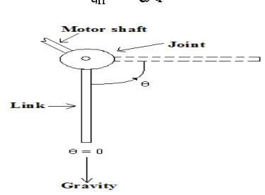
To see more clearly the effects of the gravity disturbance on robot arm joint consider Fig. 4. It is observed that initially when the joint is at = 0 rad, the gravitational force produces no additional load on the axis motor. However as  increases with time due to the command signal, the gravitational disturbance also increases and is proportional to the sine of  . For particular joint geometry, we will assume that the magnitude of this disturbance is 21oz-in. so that the time variation of gravitational torque will be

= 21

Fig. 5 Joint showing the effect of gravity as a function of 

Let the joint be initially at = 0 rad, and the desired final position of the joint be п/2 radians, so that d = /2 rad =

1.57 rad.

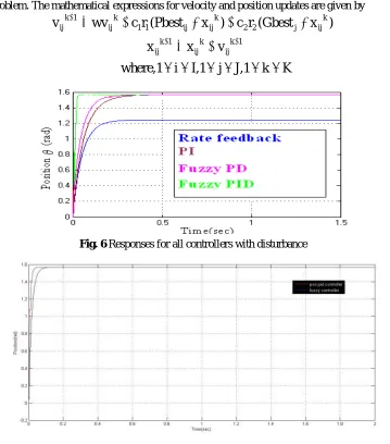
Overview of the particle swarm optimization (PSO)

(7)

their positions by “flying” around in a multidimensional search space. Particle in a swarm adjust its position in search space using its present velocity, own previous experience, and that of neighbouring particles. Therefore, a particle makes use of best position encountered by itself and that of its neighbours to steer toward an optimal solution. The performance of each particle is measured using a predefined fitness function, which quantifies the performance of the optimization problem. The mathematical expressions for velocity and position updates are given by

K

k

J,1

j

I,1

i

where,1

v

x

)

x

(Gbest

r

c

)

x

(Pbest

r

c

wv

v

1 k ij k ij 1 k ij

k ij j 2

2 k ij ij 1

1 k ij 1 k ij

















 



Fig. 6 Responses for all controllers with disturbance

Fig. 7 Response with PSO PID controller

IV. CONCLUSIONS

(8)

REFERENCES

[1] H.Ying, W.Siler, and J.J. Buckley,”Fuzzy control theory: A Non-linear case,”Automatica, vol.26, pp.513-520, 2002. [2] A. E. Hajjaji and A. Rachid, “Explicit formulas for fuzzy controller,” Fuzzy Sets Syst., vol. 62, pp. 135-141, 2000.

[3] W.Li,”Design of a hybrid fuzzy logic proportional plus conventional integral-derivative controller,” IEEE Trans. Syst., vol. 6, no. 4, pp. 449-463, Nov. 2005.

[4] G.K. Mann, B.G. Hu, and R. G. Gosine, “Analysis of direct action fuzzy PID controller structures,” IEEE Trans. Syst., Man, Cybern, B.Cybern,

vol. 29, pp.371-388, 1999.

[5] Hao Ying, “ A General Technique for Deriving Analytical Structure of Fuzzy Controllers Using Arbitrary Trapezoidal Input Fuzzy Sets and Zadeh AND Operator”. Automatica, vol .39, pp. 1171-1184, 2003.

[6] Hao Ying, “Analytical Structure of Fuzzy Controllers Using Arbitrary Input fuzzy and Zadeh Fuzzy AND operator.” Fuzzy Information, 2004.

Processing NAFIPS apos; 04. IEEE Annual Meeting of the

vol.1, Issue, 27-30 pp 276 – 280, June 2004

[7] Hao Ying “Deriving Analytical Input –Output Relationship for fuzzy controllers Using Arbitrary Input Fuzzy sets and Zadeh Fuzzy operator.”,

IEEE Transactions on Fuzzy systems Vol14, No.5, pp.654-662, October 2006

[8] K.A. Gopala Rao, K.R.Sudha “Analytical Structure of Three Input Fuzzy PID Power System Stabilizer with Decoupled Rules” WSEAS Trans. on CIRCUITS and SYSTEMS, pp.965-970, June 2004.

[9] K.A.Gopala Rao, K.R.Sudha, “Analytical Structure of PID Fuzzy Logic Power System Stabilizer Proceedings of IASTED Modeling, imulation, and Optimization MSO2004, pp143-147, August 2010.