Optimal clustering techniques for metagenomic sequencing data

(1)

Western University Western University

Scholarship@Western

Electronic Thesis and Dissertation Repository

8-2-2012 12:00 AM

Optimal clustering techniques for metagenomic sequencing data

Erik T. Cameron

The University of Western Ontario

Supervisor L. M. Wahl

The University of Western Ontario

Graduate Program in Applied Mathematics

A thesis submitted in partial fulfillment of the requirements for the degree in Master of Science © Erik T. Cameron 2012

Follow this and additional works at: https://ir.lib.uwo.ca/etd

Part of the Bioinformatics Commons

Recommended Citation Recommended Citation

Cameron, Erik T., "Optimal clustering techniques for metagenomic sequencing data" (2012). Electronic Thesis and Dissertation Repository. 707.

https://ir.lib.uwo.ca/etd/707

This Dissertation/Thesis is brought to you for free and open access by Scholarship@Western. It has been accepted for inclusion in Electronic Thesis and Dissertation Repository by an authorized administrator of

(2)

(Thesis format: Integrated Article)

by

Erik Cameron

Graduate Program in Applied Mathematics

A thesis submitted in partial fulfillment

of the requirements for the degree of

Masters of Science

The School of Graduate and Postdoctoral Studies

The University of Western Ontario

London, Ontario, Canada

c

(3)

THE UNIVERSITY OF WESTERN ONTARIO

School of Graduate and Postdoctoral Studies

CERTIFICATE OF EXAMINATION

Supervisor:

. . . . Dr. L. M. Wahl

Supervisory Committee:

Examiners:

. . . . Dr. G. Wild

. . . . Dr. X. Zou

. . . . Dr. G. Gloor

The thesis by

Erik T Cameron

entitled:

Optimal clustering techniques for metagenomic sequencing data

is accepted in partial fulfillment of the requirements for the degree of

Masters of Science

. . . . Date

. . . .

Chair of the Thesis Examination Board

(4)

Metagenomic sequencing techniques have made it possible to determine the composition of

bacterial microbiota of the human body. Clustering algorithms have been used to search for

core microbiota types in the vagina, but results have been inconsistent, possibly due to

method-ological differences. We performed an extensive comparison of six commonly-used clustering

algorithms and four distance metrics, using clinical data from 777 vaginal samples across 5

studies, and 36,000 synthetic datasets based on these clinical data. We found that

centroid-based clustering algorithms (K-means and Partitioning around Medoids), with Euclidean or

Manhattan distance metrics, performed well. They were best at correctly clustering and

de-termining the number of clusters in synthetic datasets and were also top performers for

pre-dicting vaginal pH and bacterial vaginosis by clustering clinical data. Hierarchical clustering

algorithms, particularly neighbour joining and average linkage, performed less well, failing

unequivocally on many datasets.

Keywords: vaginal microbiota, bacterial vaginosis, metagenomics, cluster analysis, distance

metric

(5)

Co-Authorship

The work presented in Chapter 2 has been submitted for publication with the title Optimal

clustering techniques for metagenomic sequencing data are predictive of clinical measures in

the vaginal microbiota and is coauthored by E. T. Cameron and L. M. Wahl. The original draft

for the article was prepared by the author and revisions were done by the author and L. M.

Wahl. The analytical work using Matlab was performed by the author under the supervision of

L. M. Wahl.

(6)

I would like thank my supervisor, Dr. Lindi Wahl, for her guidance in completing this Thesis.

You are the perfect combination of scientist, teacher, and friend and I feel lucky to have worked

with you. Your knowledge of a broad range of topics and disciplines has been invaluable and I

could not have completed this work without you. Thank you.

I would also like to thank Dr. Gregor Reid and Dr. Gregory Gloor as well as their research

groups, especially Jean Macklaim for providing access to the clinical data, and Andrew

Fer-nandes for advice regarding the clustering algorithms and distance metrics.

Finally, I would like to thank Dr. GeoffWild whose instruction and advice with the use of

LaTeX and BibTeX have been extremely helpful in the completion of this project.

(7)

List of Figures

1.1 Proportion of biota composed by the six most common OTUs . . . 12

1.2 Proportion of biota composed by a rare OTU over all profiles . . . 15

1.3 Proportion of biota composed by L. iners for one cluster . . . 15

1.4 Proportion of biota composed by L. crispatus over all profiles . . . 15

1.5 Beta probability density functions for several values of input parametersαandβ. 16 2.1 Performance of each process . . . 30

2.2 Performance of each clustering algorithm with its best distance metric . . . 31

2.3 Proportion of trials identifying the correct number of clusters by clustering algorithm . . . 32

2.4 Prediction of BV by clustering algorithm . . . 33

2.5 Prediction of pH by clustering algorithm . . . 34

3.1 Abundance comparison of common strains . . . 44

A.1 Proportion of biota composed by the six most common OTUs . . . 47

A.2 Relative Standard Deviation of each OTU . . . 48

A.3 Difference in clustering results with or without unidentified sequences . . . 49

A.4 Performance of each process on synthetic datasets of 200 compositional profiles 50 A.5 As Figure A.4, but for synthetic datasets of 50 compositional profiles. . . 51

A.6 As Figure A.4, but for synthetic datasets of 20 compositional profiles. . . 51

A.7 Performance of each process on synthetic datasets of 500 compositional pro-files for Hard Cluster Parameters . . . 52

A.11 Performance of each clustering algorithm with best distance metric on synthetic datasets of 500 compositional profiles . . . 54

A.12 Performance of each clustering algorithm assigning synthetic data to correct clusters . . . 55

A.13 Proportion of trials determining correct number of clusters in synthetic data for each clustering algorithm . . . 56

A.14 BV entropy explained by each process for pooled clinical data . . . 57

A.15 As Figure A.14, but for clinical data from the Tanzania HIV study. . . 58

A.16 As Figure A.14, but for clinical data from the Brazil BV study. . . 58

A.17 As Figure A.14, but for clinical data from the Canadian post-menopause study. . 59

A.18 As Figure A.14, but for clinical data from the Canadian preterm labour study. . 59

(10)

A.21 As Figure A.20, but for clinical data from the Tanzania HIV study. . . 62 A.22 As Figure A.20, but for clinical data from the Canadian post-menopause study. . 62

(11)

List of Tables

1.1 Summary of previous studies clustering vaginal microbiota. . . 10

(12)

Appendix A Supplementary Information . . . 46

(13)

Chapter 1 Introduction

1.1 Human Microbiota

The human microbiome is an ecosystem of microbes that colonize the human body. These

microbes can be found throughout the organs of the body such as in the intestine and vagina,

and on the surface of the skin. They play significant roles in our metabolism, helping to

di-gest food and synthesize vitamins (Guarner and Malagelada, 2003), or protect the body from

infection (Gupta et al., 1998). The living elements of a microbiome are known as microbiota.

When referring to microbiota within this text we will specifically be referring to the bacterial

elements thereof.

Previous techniques for sequencing human microbiota have relied on culturing bacteria

before sequencing genetic information (Hugenholtz, 2002). This meant that bacteria which

did not survive in cultures were missed and results were biased towards bacteria that thrived in

cultures. More recent metagenomic techniques amplify genetic material directly from samples,

without the need for an intermediate culturing step, resulting in better representation of the

microbiota associated with a sample (Hugenholtz, 2002).

High-throughput sequencing methods, such as Illumina and 454 sequencing, are common

metagenomic methods (Pareek et al., 2011; Hall, 2007). They use a set of genes referred to as

16S rDNA as a sequencing target (Case et al., 2007). This set of genes is universal and highly

conserved among bacteria and codes for the 16S ribosomal RNA subunit, which forms part

(14)

of the structure of bacterial ribosomes (Woese, 1987). 16S rDNA in the sample is amplified

and sequenced. Bacteria can be identified by matching their unique 16S rDNA sequences to a

reference database of bacterial genome sequences (Hugenholtz, 2002).

Terminal Restriction Fragment Length Polymorphism (T-RFLP) is a technique which can

be used to identify the bacteria in a sample by measuring the size of certain fragments of their

16S rDNA (Liu et al., 1997). 16S rDNA in a sample is amplified and tagged with a fluorescent

dye. Restriction enzymes are added to the solution. These are enzymes which cut DNA at a

specific sequence known as a restriction site. The chosen restriction sites are highly conserved

among most bacteria, but they occur at varying distances along the 16S gene. The result is

that each sequence is cut into a fragment whose size is characteristic of its parent bacteria (Liu

et al., 1997). The taxonomic identity of the bacteria can then be determined by comparing the

lengths of these fragments to a database.

The lengths of the fragments from a sample are determined by electrophoresis on agarose

gel. Occasionally, different bacteria produce similar length fragments when cut at a particular

restriction site. These bacteria can be distinguished by using multiple restriction enzymes

marked with different dyes in separate runs, and comparing the results using software (Liu

et al., 1997).

The results of both T-RFLP and high-throughput sequencing methods are absolute counts

for each operational taxonomic unit (OTU) identified in the sample. An OTU contains a group

of sequences which have been identified to a certain taxonomic level such as species or genus.

The level of taxonomic identification can differ throughout a dataset. The counts are

normal-ized to give an abundance profile, indicating the relative abundance of each OTU. In practice,

many sequences in a given sample will have no match in the reference database, resulting

in a certain proportion of unknown bacteria in each abundance profile (Hall, 2007).

High-throughput sequencing and T-RFLP have been used in the literature to produce abundance

profiles of microbiota in parts of the human body such as the gut (Arumugam et al., 2011),

(15)

1.1. H M 3

2007), stomach (Bik et al., 2006), and mouth (Aas et al., 2005).

Vaginal microbiota are of particular interest to researchers because of the role they play in

women’s health. Healthy vaginal microbiota maintain an acidic pH level of around 4.5, which

can help prevent urinary tract infections (Gupta et al., 1998), as well as the transmission of

human immunodeficiency virus (HIV) (Lai et al., 2009). The maintenance of this acidity is

generally attributed to the presence of lactic acid-producing bacteria in these biota (Boskey

et al., 2001).

Bacterial vaginosis (BV) is a common condition affecting about 30% of women

world-wide (Martinez et al., 2009). The condition causes unpleasant discharge and odour as well as

increased susceptibility to sexually transmitted infection (Fredricks et al., 2005). The

relation-ship between BV and vaginal microbiota has been studied by Ravel et al. (2010) who used

high-throughput 454 sequencing on 16S rRNA to profile the vaginal biota of 396 white, black,

Hispanic and Asian women living in North America. Five major community types were

iden-tified. Communities high in Lactobacillus bacteria were associated with healthy biota while

those dominated by other taxa, including Gardnerella and Atopobium were associated with BV.

Similar results were reported by Hummelen et al. (2010), who used high-throughput Illumina

sequencing to profile the vaginal biota of 132 HIV positive women in Tanzania. These authors

detected eight community types and identified Lactobacillus iners and Lactobacillus crispatus

as being associated with healthy biota while communities containing Gardnerella vaginalis

were associated with BV.

Racial differences in vaginal microbiota have been studied by Zhou et al. (2007) who

pro-filed the composition of vaginal biota in 144 North American Caucasian and black women

using T-RFLP. The authors identified 8 kinds of vaginal communities and found large

dif-ferences in the community compositions between the two racial groups, with Lactobacillus

dominated communities being rarer in black women. This difference in vaginal communities

was offered as a potential explanation for the increased susceptibility of black women to BV,

(16)

to BV (Ravel et al., 2010; Hummelen et al., 2010).

A similar study by Zhou et al. (2010) examined the abundance profiles of 73 Japanese

women using T-RFLP. Seven community types were identified, all of which were similar to

those found in black and white women in the previous study. Japanese women were more

likely than black women to have biota dominated by lactobacilli and were more resistant to

BV, supporting the vaginal community explanation for racial difference in BV susceptibility.

The researchers cited genetic differences in immune function which affect the composition of

the microbiota, as noted by Dethlefsen et al. (1987). However, for both articles (Zhou et al.,

2007, 2010) each racial group studied was represented for each vaginal community type. This

suggests that while race and genetics play primary roles in determining the biota of an

individ-ual, the same community types are shared across several geographic regions. The similarity

of these data supports the validity of combining and comparing data between studies, which

could potentially offer new insights.

1.2 Clustering

Clustering algorithms are a set of tools that are commonly used to analyze microbiota. They

aggregate abundance profiles into groups with similar bacterial compositions. An abundance

profile can be visualized as a point on a simplex with dimensionality equal to the total number

of unique OTUs identified. Profiles with similar bacterial compositions are close to each other

in the space of this simplex.

A wide variety of clustering algorithms exist for handling a large range of data types.

Clus-tering of abundance profiles has to date mostly involved the use of hierarchical clusClus-tering

algo-rithms (Ravel et al., 2010; Zhou et al., 2010; Hummelen et al., 2010), although centroid-based

methods have been used as well (Arumugam et al., 2011). Hierarchical methods are probably

the most familiar to researchers in the field because of their frequent application in the

(17)

1.2. C 5

are joined. This is repeated until the desired number of clusters is produced. Centroid-based

methods place a number of centroids in a dataset and assign each data point to the cluster

as-sociated with the closest centroid. The positions of the centroids are chosen to minimize some

objective function, such as the sum of the squared distances from each data point to its centroid.

Studies of the vaginal microbiome have used hierarchical algorithms rather than

centroid-based techniques. Algorithms used in the literature include Ward’s method (Zhou et al., 2010),

UPGMA (unweighted pair group method with arithmetic mean, also called average linkage

clustering) (Zhou et al., 2007), complete linkage clustering (Ravel et al., 2010), and neighbour

joining (Hummelen et al., 2010). A study of gut microbiota (Arumugam et al., 2011) used

Partitioning around Medoids (PAM), a centroid-based algorithm.

UPGMA clustering (Sokal and Michener, 1958) determines the closest clusters by

measur-ing the distance between every pairwise combination of points in the two clusters, and

aver-aging. The two clusters with the smallest average distance are combined. Complete linkage

clustering (Sorensen, 1948) instead measures the distance between two clusters by choosing

one data point from each cluster such that the distance between the two points is maximized.

Neighbour joining (Saitou and Nei, 1987) calculates a value between two clusters, i and j as,

D(i, j)=(n−2)d(i, j)− n

X

k=1

d(i,k)− n

X

k=1

d( j,k), (1.1)

where d(i, j) is the distance between the two clusters if they are single points, or is defined below in Equation (1.2) for clusters formed by combination at earlier steps, and n is the current

number of clusters. This value is computed for each pair of clusters to produce the matrix D.

Clusters a and b are then combined if D(a,b) is the minimal non-diagonal entry of D. The first term on the right side of Equation (1.1) causes clusters farther from each other to be less likely

to be combined. The next two terms cause clusters distant from the majority of the dataset to

be more likely to be combined. Each time a new cluster, c is created by joining two clusters a

(18)

d(c,k)= d(a,k)+d(b,k)−d(a,b)

2 . (1.2)

This distance is calculated for all remaining clusters k , _{c after each combination step so}

that the matrix D can be calculated according to Equation (1.1) in the next step.

Ward’s method (Ward, 1963) considers each possible ‘next step’ of combined clusters. For

each, it calculates the sum of the squared distances (S S D) from the each data point, j, to the

center (mean) of its cluster, mj. For a dataset with N abundance profiles this is expressed as,

S S D=

N

X

j=1

d( j,mj)2. (1.3)

At each step, Ward’s method combines the two clusters which will reduce the SSD of the

dataset by the greatest amount.

Centroid-based methods place a set of K centroids in the space of a dataset to produce an

aggregation of K clusters. They assign each data point to the cluster associated with the closest

centroid, and calculate the S S D from each data point, j, to its cluster centroid cj, using the

same calculation as in Equation (1.3) while replacing mj by cj. The solution when using the

K-means (Lloyd, 1982) and PAM (Kaufman and Rousseeuw, 1990) clustering algorithms is the

placement of centroids which minimizes this S S D. While there is a single optimal solution to

these clustering results, calculating it directly is computationally complex (MacQueen, 1967).

Instead, heuristic algorithms which randomly place the initial centroids and recursively move

them through the space of the dataset are used. Each step moves a single centroid so that the

S S D of the system is reduced, and the algorithm ends when the S S D cannot be reduced in a

further step (MacQueen, 1967). K-means clustering (Lloyd, 1982) moves the centroids through

continuous space while PAM (Kaufman and Rousseeuw, 1990) moves them only into positions

occupied by data points.

The heuristic algorithms used to solve K-means and PAM clustering are non-deterministic.

(19)

1.2. C 7

movement step, they will return it as the solution to the clustering problem even if it is not

the absolute minimum solution (MacQueen, 1967). To achieve a result close to the absolute

minimum, several runs of the clustering algorithm are typically used, each with a different

random initial placement of centroids. The run which produces the lowest S S D is taken as the

best solution.

When a clustering algorithm is used, a distance metric must be chosen to define the distance

between two points in the space of a dataset. The most familiar distance metric is Euclidean

distance, which defines the distance between two vectors, v and u, using a generalization of the

Pythagorean Theorem,

Euclidean distance (v,u)= p(v−u)·(v−u). (1.4)

The Euclidean distance metric has been used for clustering in research on the microbiota

of the human gut (Arumugam et al., 2011) and vagina (Zhou et al., 2007). Similar distance

metrics include Manhattan distance, which defines the distance between two points as the sum

of the difference in position along each axis, similar to a measure of distance for a trip along

city streets which form a grid. For vectors v and u in n dimensions it uses the formula

Manhattan distance (v,u)=

n

X

i=1

|vi−ui|. (1.5)

Distances can also be defined by the angle between two vectors. If the angle between v and

u isθ, then the cosine distance between the vectors is defined as,

Cosine Distance (v,u)=1−cos (θ). (1.6)

This distance metric has been used for clustering in research of the microbiota of the human

(20)

Correlation between the elements of two vectors, Correlation (v,u),

Correlation Distance (v,u)=1−Correlation (v,u), (1.7)

which has also been used in research clustering human vaginal microbiota (Zhou et al., 2010).

Cluster optimization is the practice of determining the number of clusters in a real dataset.

Clustering algorithms produce a number of clusters determined a priori by the investigator.

There are several objective techniques that can be used to select a number of clusters to

pro-duce from a real dataset. Research on vaginal microbiota has used objective methods such as

the Pseudo-F index of Calinski and Harabasz (1974) in some studies (Zhou et al., 2007, 2010)

while others have not indicated the methods of optimization used (Ravel et al., 2010;

Humme-len et al., 2010). This issue has been studied in detail by Abdo et al. (2006), who recommended

three objective techniques for cluster optimization of abundance profile data. Of these three we

use the Pseudo-F index of Calinski and Harabasz (1974). This technique requires the user to

create a large range of numbers of clusters, and produces a score for each aggregation which

indicates how well the spatial variance is explained with as few clusters as possible (Calinski

and Harabasz, 1974). The user keeps the aggregation with the highest score.

High-dimensional data can cause clustering algorithms to fail to produce meaningful

re-sults. This ‘curse of dimensionality’ occurs when data points are distributed over a space

with a very large number of dimensions. The distance between any two points in a space will

increase with the number of dimensions and the distance between two clusters which differ

in only a few dimensions becomes relatively small (Steinbach et al., 2003). This obfuscates

clusters in the data and many clustering algorithms will not properly detect them (Aggarwal

et al., 1999). Solutions include using feature selection to remove noisy dimensions from the

data before clustering, or employing clustering algorithms that project clusters into the relevant

dimensions (Aggarwal et al., 1999).

(21)

1.3. O C 9

dimensionality and group correlated variables, and is often applied to data before clustering

(Ding and He, 2004). It is useful for removing noise from data and has been shown to improve

the performance of the K-means clustering algorithm on some datasets, helping to find

solu-tions that are closer to optimal (Ding and He, 2004). Pre-treatment of data with PCA has been

used in one study of human gut microbiota which was then clustered using PAM (Arumugam

et al., 2011).

In summary, to cluster a set of data, a clustering technique and distance metric must first be

chosen. The number of clusters can then be determined using an optimization technique. The

data may or may not be pre-treated with techniques such as PCA.

1.3 Our Contribution

As the tools of microbiome analysis improve and a growing amount of research examines the

composition of the human vaginal microbiome, it is clear that using effective data analysis

techniques is of increasing importance. Many studies of the human microbiome use cluster

analysis to group similar abundance profiles, including several studies of vaginal microbiota

(Zhou et al., 2010, 2007; Ravel et al., 2010; Hummelen et al., 2010) and a landmark study

investigating microbiota of the human gut (Arumugam et al., 2011). Clustering is used to

group subjects with similar abundance profile composition. In the gut microbiota study by

Arumugam et al. (2011) the investigators found three clusters which they called enterotypes.

Similar efforts with vaginal microbiota have yielded as few as five (Ravel et al., 2010) or as

many as 12 (Zhou et al., 2007) clusters, as shown on Table 1.1. This research has relied on a

variety of methodologies, including differences in clustering algorithms, distance metrics, and

cluster optimization. Our goal is to recommend a single, consistent technique for the treatment

(22)

Table 1.1: Summary of previous studies clustering vaginal microbiota.

Study # Sequencing Cluster Technique, Cluster #

Profiles Technique Distance Metric Optimization Clusters

Zhou et al. 144 T-RFLP UPGMA, Calinski- 12

2007 Euclidean Harabasz

Zhou et al. 73 T-RFLP Ward’s Method, Calinski- 9

2010 Correlation Harabasz

Ravel et al. 396 High-through Complete Linkage, Not 5

2010 (454) Euclidean Declared

Hummelen 132 High-through Neighbour joining, Not 8

(23)

1.3. O C 11

Our primary objective is to find a data analysis technique that groups patients into

bio-logically relevant clusters. For example, several studies of vaginal microbiota have had an

emphasis on subjects with BV (Martinez et al., 2008; Hummelen et al., 2010; Ravel et al.,

2010). A tool that consistently clusters subjects into groups which are predictive of BV status

would be useful. Similarly, the clusters we find should be able to predict vaginal pH, which is

an indicator of vaginal health (Gupta et al., 1998).

We prefer to recommend techniques that are easy to execute and interpret. For this reason

we focus on clustering techniques that are widely available in software packages such as R and

Matlab, and can be carried out quickly on large datasets using personal computers. We focus

on sharp clustering techniques, which assign patients definitively to clusters on a one-to-one

basis, because such classifications are convenient to work with for both mathematicians and

biologists.

We use data collected in five clinical studies of vaginal microbiota in Tanzania, Brazil

and Canada, totalling 777 abundance profiles. These data included women with a variety of

health conditions such as HIV (Hummelen et al., 2010), BV or Vulvovaginal candidiasis (VVC)

(Martinez et al., 2009), as well as post-menopausal women (Hummelen et al., 2011), pregnant

women (unpublished data) and women suffering from toxin shock (unpublished data).

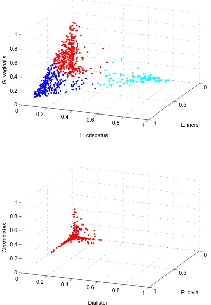
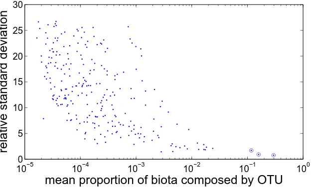
The abundance profile data that we studied had 260 unique OTUs (dimensions) but only

a few of these OTUs composed a large proportion of any abundance profiles, hence the data

were only widely distributed over the space of a few dimensions. Other papers in the

litera-ture report similar distributions in abundance profile data (Ravel et al., 2010; Martinez et al.,

2008). Preliminary trials with these data indicated that basic clustering techniques used for low

dimensional data, such as K-means, could produce meaningful clustering results. For this

rea-son our investigation did not focus on clustering techniques designed to treat high-dimensional

data, which are most useful where basic clustering algorithms fail and when data are widely

distributed over many dimensions (Aggarwal et al., 1999). Figure 1.1 shows the distribution of

(24)

0

0.5

1 0

0.2 _0.4 0.6

0.8 ₁ 0

0.2 0.4 0.6 0.8 1

L. iners L. crispatus

G. vaginalis

0

0.5

1 0 _0.2

0.4

0.6 _0.8 1 0

0.2 0.4 0.6 0.8 1

P. bivia Dialister

Clostridiales

(25)

1.3. O C 13

PCA has been used in the literature to treat abundance profile data before clustering

(Aru-mugam et al., 2011) and has been shown to improve the performance of K-means in some cases

(Ding and He, 2004). Preliminary tests on our clinical data showed that for the pooled set of

777 abundance profiles, the clustering result for K-means with 10 replicates was identical with

or without the application of PCA to the data. We chose not pre-treat our data with PCA before

clustering because it did not have an impact on results, and to reduce the complexity of our

data analyses.

Ultimately we tested six clustering algorithms and four distance metrics. We tested the

UP-GMA, Ward’s method, neighbour joining and complete linkage hierarchical clustering

algo-rithms, and the K-means and PAM centroid-based clustering methods. We used the Euclidean,

Manhattan, cosine and correlation distance metrics. Clustering requires a choice of algorithm

and distance metric, giving us a total of 24 algorithm-metric combinations which we refer to

as processes.

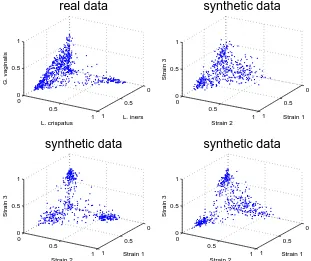
We generated 36,000 synthetic abundance profiles based on our clinical data. Frequency

distributions for OTUs in the real data tended to be single peaked within clusters but some

were double peaked over the entire dataset (examples can be seen in Figures 1.2 to 1.4). We

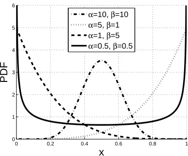
chose to use the beta distribution to generate these data. The beta distribution has two positive

parameters,αandβ, and generates a value from 0 to 1. It can generate single peaked distribu-tions which form a ‘hump’ similar to a Gaussian, or are monotonically decreasing or increasing

with a peak at 0 or 1 respectively, similar to an exponential distribution. It can also generate

double peaked distributions which tend towards values of 0 and 1. Figure 1.5 shows example

probability density functions (PDFs) for the beta distribution.

We found that the single peaked beta distributions emulated common OTUs well, as was

the case in Figure 1.3. They emulated rare OTUs like that in Figure 1.2 well when they took on

an exponential-like shape with a maximum at 0. For OTUs which had frequency distributions

with two peaks, a double peaked beta distribution was effective as shown in Figure 1.4.

(26)

profiles. We fit these distributions to each OTU over the dataset as a whole to generate noise.

We also partitioned our dataset into three clusters using K-means and fit beta distributions for

each OTU within the separate clusters. These three sets of distributions were used to generate

clustered data. Figures 1.2 to 1.4 show the frequency distributions for some OTUs in real data,

and compares them to the distributions for synthetic OTUs which were based on them. For

additional details on the production of synthetic data see the Methods section in the following

chapter.

We tested which processes were best at determining the true number of clusters, and

cor-rectly clustering these synthetic data. For our clinical data, we tested which processes were

(27)

1.3. O C 15

0 0.1 0.2 0.3 0.4 0.5 0 0.05 0.1 0.15 0.2 0.25 0.3 0.35 0.4 0.45 0.5 frequency

proportion of biota real data

0 0.1 0.2 0.3 0.4 0.5 0 0.05 0.1 0.15 0.2 0.25 0.3 0.35 0.4 0.45 0.5

proportion of biota synthetic data

Figure 1.2: Proportion of biota composed by a rare OTU over all profiles

0 0.2 0.4 0.6 0.8 1 0 0.02 0.04 0.06 0.08 0.1 0.12 0.14 0.16 0.18 0.2 frequency

0 0.2 0.4 0.6 0.8 1 0 0.02 0.04 0.06 0.08 0.1 0.12 0.14 0.16 0.18 0.2

Figure 1.3: Proportion of biota composed by L. iners for one cluster

0 0.2 0.4 0.6 0.8 1 0 0.1 0.2 0.3 0.4 0.5 0.6 0.7 frequency

0 0.2 0.4 0.6 0.8 1 0 0.1 0.2 0.3 0.4 0.5 0.6 0.7

(28)

0 0.2 0.4 0.6 0.8 1 0

1 2 3 4 5 6

x

PDF

α=10, β=10

α=5, β=1

α=1, β=5

α=0.5, β=0.5

(29)

BIBLIOGRAPHY 17

Bibliography

Aas, J. A., Paster, B. J., Stokes, L. N., Olsen, I., and Dewhirst, F. E. (2005). Defining the normal bacterial flora of the oral cavity. J. Clin. Microbiol., 43(11):5721–5732.

Abdo, Z., Schuette, U., Bent, S., Williams, C., Forney, L., and Joyce, P. (2006). Statistical methods for characterizing diversity of microbial communities by analysis of terminal re-striction fragment length polymorphisms of 16S rRNA genes. Environ Microbiol., 8(5):929– 938.

Aggarwal, C. C., Wolf, J. L., Yu, P. S., Procopiuc, C., and Park, J. S. (1999). Fast algorithms for projected clustering. SIGMOD Rec., 28(2):61–72.

Arumugam, M., Raes, J., Pelletier, E., Paslier, D. L., Yamada, T., Mende, D., Fernandes, G., Tap, J., Bruls, T., Batto, J.-M., Bertalan, M., Borruel, N., Casellas, F., Fernandez, L., Gautier, L., Hansen, T., Hattori, M., Hayashi, T., Kleerebezem, M., Kurokawa, K., Leclerc, M., Levenez, F., Manichanh, C., Nielsen, H., Nielsen, T., Pons, N., Poulain, J., Qin, J., Sicheritz-Ponten, T., Tims, S., Torrents, D., Ugarte, E., Zoetendal, E., Wang, J., Guarner, F., Pederson, O., de Vos, W., Brunak, S., Dore, J., Weissenbach, J., Ehrlich, S., and Bork, P. (2011). Enterotypes of the human gut microbiome. Nature, 473:174–180.

Bik, E. M., Eckburg, P. B., Gill, S. R., Nelson, K. E., Purdom, E. A., Francois, F., Perez-Perez, G., Blaser, M. J., and Relman, D. A. (2006). Molecular analysis of the bacterial microbiota in the human stomach. Proc Nat Acad Sci USA, 103(3):732–737.

Boskey, E., Cone, R., Whaley, K., and Moench, T. (2001). Origins of vaginal acidity: high D/L lactate ratio is consistent with bacteria being the primary source. Hum. Reprod., 16(9):1809– 1813.

Calinski, T. and Harabasz, J. (1974). A dendrite method for cluster analysis. Commun Stat, 3(1):1–27.

Case, R. J., Boucher, Y., Dahllf, I., Holmstrm, C., Doolittle, W. F., and Kjelleberg, S. (2007). Use of 16S rRNA and rpoB genes as molecular markers for microbial ecology studies. Appl. Environ. Microbiol., 73(1):278–288.

Dethlefsen, L., McFall-Ngai, M., and Relman, D. A. (1987). An ecological and evolutionary perspective on humanmicrobe mutualism and disease. Nature, 449:811–818.

Ding, C. and He, X. (2004). K-means clustering via principle component analysis. In Proc. of Int’l Conf. Machine Learning, pages 225–232.

Fredricks, D. N., Fiedler, T. L., and Marrazzo, J. M. (2005). Molecular identification of bacteria associated with bacterial vaginosis. N. Engl. J. Med., 353(18):1899–1911.

(30)

Gupta, K., Stapleton, A., Hooton, T., Roberts, P., Fennell, C., and Stamm, W. (1998). In-verse association of h2o2-producing lactobacilli and vaginal Escherichia coli colonization in women with recurrent urinary tract infections. J Infect Dis, 178(2):446–450.

Hall, N. (2007). Advanced sequencing technologies and their wider impact in microbiology. J. Exp. Biol., 209:1518–1525.

Hugenholtz, P. (2002). Exploring prokaryotic diversity in the genomic era. Genome Biol., 3(2):reviews0003.1–reviews0003.8.

Hummelen, R., Fernandes, A. D., Macklaim, J. M., Dickson, R. J., Changalucha, J., Gloor, G. B., and Reid, G. (2010). Deep sequencing of the vaginal microbiota of women with HIV. PLoS ONE, 5(8):e12078.

Hummelen, R., Macklaim, J. M., Bisanz, J. E., Hammond, J.-A., McMillan, A., Vongsa, R., Koenig, D., Gloor, G. B., and Reid, G. (2011). Vaginal microbiome and epithelial gene array in post-menopausal women with moderate to severe dryness. PLoS ONE, 6(11):e26602.

Kaufman, L. and Rousseeuw, P. (1990). Finding groups in data: an introduction to cluster analysis. Wiley series in probability and mathematical statistics: Applied probability and statistics. Wiley.

Lai, S. K., Hida, K., Shukair, S., Wang, Y.-Y., Figueiredo, A., Cone, R., Hope, T. J., and Hanesl, J. (2009). Human immunodeciency virus type 1 is trapped by acidic but not by neutralized human cervicovaginal mucus. J. Virol., 83(21):11196–11200.

Liu, W., Marsh, T., Cheng, H., and Forney, L. (1997). Characterization of microbial diversity by determining terminal restriction fragment length polymorphisms of genes encoding 16S rRNA. Appl. Environ. Microbiol., 63(11):4516–4522.

Lloyd, S. P. (1982). Least squares quantization in PCM. IEEE Trans Inf Theory, 28(2):129– 137.

MacQueen, J. B. (1967). Some methods for classification and analysis of multivariate observa-tions. In Proceedings of 5th Berkeley Symposium on Mathematical Statistics and Probability. University of California Press, pages 281–297.

Martinez, R. C. R., Franceschini, S. A., Patta, M. C., Quintana, S. M., Gomes, B. C., Mar-tinis, E. C. P. D., and Reid., G. (2009). Improved cure of bacterial vaginosis with single dose of tinidazole (2 g), Lactobacillus rhamnosus gr-1, and Lactobacillus reuteri rc-14: a randomized, double-blind, placebo-controlled trial. Can J Microbiol, 55(2):133–138.

Martinez, R. C. R., Franceschini, S. A., Patta, M. C., Quintana, S. M., Nunes, A. C., Mor-eira, J. L. S., Anukam, K. C., Reid, G., , and Martinis, E. C. P. D. (2008). Analysis of vaginal lactobacilli from healthy and infected Brazilian women. Appl. Environ. Microbiol., 74(14):4539–4542.

(31)

BIBLIOGRAPHY 19

Ravel, J., Gajer, P., Abdo, Z., Schneider, G. M., Koenig, S. S. K., McCulle, S. L., Karlebach, S., Gorle, R., Russell, J., Tacket, C. O., Brotman, R. M., Davis, C. C., Ault, K., Peralta, L., and Forney, L. J. (2010). Vaginal microbiome of reproductive-age women. Proc Nat Acad Sci USA, 108:4680–4687.

Saitou, N. and Nei, M. (1987). The neighbor-joining method: a new method for reconstructing phylogenetic trees. Mol. Biol. Evol., 4(4):406–425.

Sokal, R. R. and Michener, C. D. (1958). A statistical method for evaluating systematic rela-tionships. University of Kansas Science Bulletin, 38:1409–1438.

Sorensen, T. (1948). A method of establishing groups of equal amplitude in plant sociology based on similarity of species content and its application to analyses of the vegetation on Danish Commons. Biologiske Skrifter, 5:1–34.

Steinbach, M., Ertz, L., and Kumar, V. (2003). The challenges of clustering high-dimensional data. In In New Vistas in Statistical Physics: Applications in Econophysics, Bioinformatics, and Pattern Recognition. Springer-Verlag.

Ward, J. H. (1963). Hierarchical grouping to optimize an objective function. JASA, 58(301):236–244.

Woese, C. R. (1987). Bacterial evolution. Microbiol. Mol. Biol. Rev., 51(2):221–271.

Zhou, X., Brown, C., Abdo, Z., Davis, C., Hansmann, M., Joyce, P., Foster, J., and Forney, L. (2007). Differences in the composition of vaginal microbial communities found in healthy Caucasian and black women. ISME J., 1:121–133.

(32)

Optimal clustering techniques for vaginal

microbiota

2.1 Introduction

In the last decade, interest in the bacterial populations (microbiota) of the human body has been

growing. Advances in metagenomic sequencing techniques have made possible the collection

of the rich datasets needed to characterize the composition of these populations. For example,

recent efforts have been made to characterize microbiota within the human gut (Arumugam

et al., 2011); similar efforts have also been directed toward the characterization of microbiota

of the stomach (Bik et al., 2006) and oral cavity (Aas et al., 2005). Vaginal microbiota have

been a focus of particular recent interest (Ravel et al., 2010; Hummelen et al., 2010; Martinez

et al., 2008; Zhou et al., 2007, 2010).

2.1.1 Composition of Microbiota

Modern metagenomic sequencing techniques amplify bacterial genetic elements directly from

a sample (Hugenholtz, 2002), such as a faecal sample or vaginal swab. Two common

metage-nomic techniques that identify the bacterial compositions of biota are high-throughput

sequenc-ing, and Terminal Restriction Fragment Length Polymorphism (T-RFLP). High-throughput

techniques copy and sequence a highly conserved, universal gene. These are then identified

(33)

2.1. I 21

by comparison to a database of previously sequenced bacterial genomes (Hugenholtz, 2002).

In T-RFLP, DNA is cut at common, highly conserved sites and the lengths of the resulting

fragments are measured. They are then identified by comparison to a database of previously

cut bacterial genomes (Liu et al., 1997). For both techniques, the result is an absolute count of

the number of reads for each operational taxonomic unit (OTU) in the sample. The counts are

normalized giving an abundance profile indicating the proportion of each OTU in the sample.

An abundance profile can be represented as a point on a simplex whose dimensionality is

equal to the total number of unique OTUs detected over all samples. To reduce dimensionality

and improve understanding, a clustering algorithm is typically applied to these data. Clustering

is used to group points that are close to each other on the simplex so as to identify samples

composed of similar bacterial OTUs. The objective is to categorize subjects in ways that are

interesting or useful, for example, to identify if a set of core types (clusters) dominate the biota,

and how they relate to the health of the subject (Ravel et al., 2010). Similar attempts have been

made with gut microbiota, for which one study found 3 core types (Arumugam et al., 2011).

Results in clustering vaginal microbiota have been inconsistent, identifying as few as 5 (Ravel

et al., 2010), or as many as 12 (Zhou et al., 2007) clusters in the data. However, since an

established method for clustering and analysis of abundance profile data has yet to emerge,

methodological differences could underlie these inconsistencies.

2.1.2 Clustering

Two broad categories of clustering algorithms have been applied to abundance profile data

to date: hierarchical and centroid-based. Hierarchical methods treat each data point as an

individual cluster and recursively combine the closest ones until the desired number of clusters

is reached. Centroid-based methods place one centroid in the data space for each desired

cluster. Each data point is then assigned to the cluster corresponding to the closest centroid.

The centroids are recursively moved to minimize some objective function, such as the sum of

(34)

objective function cannot be lowered by another step.

Because finding the optimal solution for a centroid-based method is computationally

ex-pensive, a heuristic algorithm is used, making the outcome non-deterministic. The outcome

can depend on the initial, random placements of centroids in the dataset, and a single run of

the algorithm might find a local minimum of the objective function, rather than the global

min-imum. To minimize this effect it is common practice to use multiple runs of the algorithm and

take the result which minimizes the objective function.

To date, studies of the vaginal microbiome have used hierarchical algorithms such as

Ward’s method (Zhou et al., 2010), UPGMA (unweighted pair group method with arithmetic

mean, also called average linkage clustering) (Zhou et al., 2007), complete linkage clustering

(Ravel et al., 2010), and neighbour joining trees (Hummelen et al., 2010), while the gut

mi-crobiota study (Arumugam et al., 2011) used Partitioning around Medoids (PAM), a

centroid-based algorithm.

In addition to these algorithmic differences, the distance metric, the measure used by the

algorithm to define the distance between two data points, also varies widely. Euclidean distance

is the familiar metric used in everyday measurement of distance. It has been used to cluster

gut microbiota (Arumugam et al., 2011). Angular distance measures the angle between two

points from the origin. Correlation distance takes each point in its vector form and measures

the correlation between the elements of the two vectors. Two points on a simplex that are not

equal will always have a non-zero angular and correlation distance between them. Studies of

vaginal microbiota have used Euclidean distance (Ravel et al., 2010; Zhou et al., 2007), angular

distance (Hummelen et al., 2010) and correlation distance (Zhou et al., 2010).

A final methodological issue in clustering abundance profile data is to determine the

op-timal number of clusters. Most clustering algorithms take as input a dataset and an integer

number of desired clusters and give as output a partitioning of that dataset into the same

num-ber of clusters. The numnum-ber of clusters must be chosen a priori even though the true numnum-ber of

(35)

2.1. I 23

to repeat the clustering algorithm for a large range of numbers of clusters and choose the best

result. The best result can be chosen subjectively, or through a variety of objective methods

which optimize a function, usually by finding a partitioning that best explains the spatial

vari-ance of the data with as few clusters as possible. Abdo et al. (2006) have already addressed

this issue in some detail, suggesting three algorithms that can be used to determine the optimal

number of clusters in abundance profile data.

2.1.3 Our Contribution

The vaginal microbiome plays an important role in women’s health. Bacterial vaginosis (BV)

is a common condition affecting about 30% of women worldwide and is strongly linked to

compositional changes in the subject’s vaginal microbiota (Martinez et al., 2009). Microbiota

also play a role in the resistance to yeast infections, HIV (Human Immunodeficiency Virus)

and other sexually transmitted infections (Ravel et al., 2010). To better understand the rich

datasets currently becoming available, establishing a consistent, well-studied methodology for

the clustering and analysis of microbiota data is clearly necessary.

Here, we test 24 combinations of clustering algorithms and distance metrics to find which

provide the most meaningful analyses of abundance profile datasets. We use data collected

in five clinical studies of vaginal microbiota in Tanzania, Brazil and Canada, totalling 777

abundance profiles, each characterized by 260 OTUs. We generate 36,000 synthetic data sets

with known clusters based on these clinical data. We use these synthetic data to test which

combinations are best at correctly determining the number of clusters in a dataset, and best at

assigning abundance profiles to the correct clusters. We then determine which combinations

(36)

2.2 Methods

2.2.1 Clustering

We tested two centroid-based clustering algorithms and four hierarchical clustering algorithms.

The hierarchical algorithms we tested were UPGMA, neighbour joining, Ward’s method and

complete linkage clustering. Complete linkage and UPGMA both measure the distance

be-tween two clusters to determine which two are closest. For clusters containing multiple points,

UPGMA uses the average pairwise distance between all combinations of points in the two

clus-ters (Sokal and Michener, 1958), while complete linkage uses the greatest distance between any

two points in the clusters (Sorensen, 1948). Neighbour joining uses a special distance

calcula-tion, which incorporates the distance between the two clusters, but also applies a term which

favours linking clusters far from the center of the dataset (Saitou and Nei, 1987). Finally,

Ward’s method calculates the sum of the squared distance from each point to the mean position

of the cluster it belongs to and connects the two clusters which minimize the sum of squared

distances in the next step (Ward, 1963).

The centroid-based algorithms we tested the K-means and PAM. Both algorithms attempt

to minimize the sum of squared distances from the data points to the centroids. K-means

recur-sively moves the centroids through continuous space (Lloyd, 1982), while for PAM only the

positions of data points qualify as potential positions for centroids (Kaufman and Rousseeuw,

1990). For both algorithms the centroid movement steps repeat until the sum of squared

dis-tances cannot be lowered in the next step.

To mitigate the issue of centroid-based methods finding local minima, we used 10 runs with

K-means and 15 with PAM and selected the result with the lowest sum of squared distances.

These numbers of runs were selected to consistently produce good clusterings (based on initial

observations using up to 50 runs) while minimizing computational load.

We also tested four distance metrics: Euclidean distance, Manhattan distance (also called

(37)

dis-2.2. M 25

tance are simple distance metrics that use the following formulas to give the distance between

two points in n-dimensional space with vector positions v and u,

Euclidean distance (v,u)= p(v−u)·(v−u), (2.1)

Manhattan distance (v,u)=

n

X

i=1

|ui−vi|. (2.2)

The cosine distance between two points grows as the angle between them increases, measured

from the origin. It is given as

Cosine Distance (v,u)=1−cos (θ), (2.3)

where θ is the angle between v and u. Finally, the correlation distance between two points grows as the correlation between the elements of those points shrinks. It is measured,

Correlation Distance (v,u)=1−Correlation (v,u). (2.4)

Each clustering algorithm and distance metric can be combined into a metric/algorithm

combination which we will refer to as a process. We tested four distance metrics and six

algorithms, giving a total of 24 processes.

2.2.2 Synthetic Data

To produce synthetic data, we first grouped subjects in the clinical data into 2 to 12 clusters

using K-means clustering with Euclidean distance, and used the technique of Calinski and

Harabasz (1974) to determine the optimal number of clusters. This yielded 3 clusters which

we used as a basis for generating our synthetic data. Each of the three clusters emphasized a

single dominant OTU which composed between 20% and 80% of the microbiota, while other

OTUs composed less than 40% of the biota and were often much rarer. Within each cluster,

(38)

the abundance values of all subjects for each OTU. This gave three sets of Cluster Parameters,

each consisting of 260 beta distributions corresponding to the 260 OTUs. A fourth set of beta

distributions was fitted to each OTU in the entire unclustered dataset. This set was called the

Noise Parameters.

A set of synthetic data contained K clusters and N subjects. To generate a synthetic cluster,

we selected one of the three sets of cluster parameters (randomly, with replacement) on which

the cluster would be based. Each subject in a synthetic cluster had an abundance profile based

on their cluster’s respective cluster parameters. The nth OTU was always the most common for

the nth synthetic cluster. We accomplished this by switching the nth beta distribution with the

beta distribution having the highest mean in the chosen set of cluster parameters. For example,

to generate the fourth cluster in a synthetic dataset we would randomly select one set of cluster

parameters. The beta distribution for the most common OTU in that set of cluster parameters

would be switched with the beta distribution for the fourth OTU, so that the fourth synthetic

cluster would have high amounts of OTU four. This was done so that any number of unique

synthetic clusters could be drawn from three sets of cluster parameters. To produce a synthetic

abundance profile within a cluster, the value for each OTU was drawn from the corresponding

beta distribution in the appropriate set of cluster parameters. This gave each of the 260 OTUs a

value between 0 and 1. The profile was then normalized to sum to 1. We assigned 2N₃ subjects

to clusters, yielding 2N_3K per cluster. Finally, N₃ of the subjects were assigned to the Noise Group.

Abundance profiles for the Noise Group were drawn from the noise parameters. Synthetic

datasets were produced with N =20,50,200 or 500 subjects, and with K =2 to 9 clusters. We produced 500 replicates for each combination.

For a side-by-side comparison of abundance for several OTUs in real and synthetic data,

see section A.2.7.

We used the synthetic datasets to test which processes were best at determining the true

number of clusters in a dataset. Each process was used to produce aggregations of 1 to 15

(39)

2.2. M 27

Pseudo-F method proposed by Calinski and Harabasz (1974), as recommended by Abdo et al.

(2006). A trial was considered successful if the optimal number of clusters was equal to the

true number of clusters, or the true number of clusters plus one (allowing for the identification

of noise data as a separate cluster).

We also used the synthetic datasets to test which processes were best at assigning subjects

to the correct clusters. To do this, we used each process to create an aggregation for the true

number of clusters. We then determined the conditional entropy of the true clusters given the

found clusters, H(T|F) using Shannon Entropy (Shannon, 1948). In order to produce a more

intuitive measure of entropy, and allow comparison of results, we converted this value into the

proportion of entropy explained by the clustering result, PE, which we defined as

PE = H(T )−H(T|F)

H(T ) , (2.5)

where H(T ) is the entropy of the true clusters alone. A higher value for PE indicates a better

clustering result. A result of PE = 1 indicates that every point was assigned to the correct

cluster, and a result of PE ≈ 0 indicates a highly random clustering containing little or no

information. Note that in this calculation, the synthetic data points in the Noise Group were

omitted, so as not to reward or punish an algorithm for how it classified the noise data.

We repeated the above procedures using a set of Hard Cluster Parameters designed to

produce clusters with more overlap to determine which processes were best for less easily

clustered datasets (see section A.1.1). We also produced an alternate set of cluster parameters

based on clusters found with complete linkage clustering rather than K-means. Using these

parameters we generated new synthetic datasets and tested each clustering algorithm with

Eu-clidean distance. This was used as a control to ensure that the algorithm used to generate the

cluster parameters would not bias the results. In total we generated and tested 36,000 synthetic

datasets.

(40)

obtained by clustering the same data randomly. The random clustering algorithm assigned data

points independently to each of the N clusters with probability _N1.

2.2.3 Clinical Data

We used data from five clinical studies. This included data from women with HIV from

Tan-zania (Hummelen et al., 2010) and women with or without BV and with or without yeast

infections from Brazil (Martinez et al., 2009), as well as post-menopausal women (Hummelen

et al., 2011), pregnant women (unpublished data) and women suffering from toxin shock

(un-published data) in Canada. Abundance profile data as well as a clinical diagnosis for BV was

available for all women in these studies, and a measure of vaginal pH was available in some

studies. Vaginal pH is relevant to women’s health and a higher pH is associated with BV (Zhou

et al., 2007). We evaluated the conditional entropy of the pH (increments of 0.5 from 3.5 to

8.5) given the clusters found. We also evaluated the conditional entropy of each subject’s BV

status (normal, intermediate, and BV) given the clusters found. Sufficient data concerning pH

was recorded for 344 of the abundance profiles and sufficient data concerning BV was recorded

for 668 of the abundance profiles.

We tested each process for K =2 to 9 clusters. We determined the conditional entropy of

the vaginal pH and BV status given the found clusters, H(BV|F) and H(pH|F). BV status was

determined using the Nugent Criteria (Nugent et al., 1990). Similar to our treatment of entropy

with synthetic data, we converted this value into the proportion of entropy explained by the

clustering result, which is defined as

PEBV =

(H(BV)−H(BV|F))

H(BV) for BV data and, (2.6)

PEpH =

(H(pH)−H(pH|F))

H(pH) for pH data, (2.7)

where H(pH) and H(BV) are the entropies of the BV and pH labels respectively. Again,

(41)

2.3. R 29

explanation of the clinical criteria through clustering. We tested the combined dataset from all

5 studies. We also tested the five studies with sufficient data on BV status and the two studies

with sufficient data on pH status individually. We used bootstrapping to find a 95% confidence

interval for our PE values (see section A.1.2).

2.2.4 Software

All of the algorithms we tested are available in version 7.12.0 of Matlab (The MathWorks, Inc.).

To perform K-means and neighbour joining clustering, we usedkmeans.mandseqneighjoin.m

respectively. To perform UPGMA, complete linkage and Ward’s method we usedlinkage.m.

To perform PAM clustering we usedkmedoids.mavailable on the Matlab file exchange

(http://www.mathworks.com/matlabcentral/fileexchange/28860-kmedioids

/content/kmedioids.m).

Optimization of clustered results was carried out using the Cluster Validity Analysis Platform

available on the Matlab file exchange

(http://www.mathworks.com/matlabcentral/fileexchange/14620).

2.3 Results

2.3.1 Synthetic Data

Figure 2.1 shows how well each process assigned synthetic data points to the correct cluster,

in-dicating the PE for each process. Euclidean distance worked best with UPGMA and PAM, and

Manhattan distance was best with K-means, Ward’s method and neighbour joining. No single

distance metric was clearly best for complete linkage clustering, though correlation distance

did well. The results did not conflict for smaller sample sizes (Figures A.4 to A.6). All

pro-cesses performed better than random clusters used as a control, which yielded a PE of 0.05 or

(42)

2 3 4 5 6 7 8 9 0.8

0.9

1 _K−Means

proportion of entropy explained

2 3 4 5 6 7 8 9 0.8

0.9

1 _PAM

2 3 4 5 6 7 8 9 0.8

0.9

1 _{Ward’s Method}

2 3 4 5 6 7 8 9 0.7

0.8 0.9

1 _UPGMA

2 3 4 5 6 7 8 9 0.7

0.8 0.9

1 _{Complete Linkage}

true number of clusters

2 3 4 5 6 7 8 9 0.2

0.6

1 _{Neighbour Joining}

Figure 2.1: Performance of each process on synthetic datasets of 500 abundance profiles with 2 to 9 true clusters. The PE is plotted against the number of synthetic clusters in the dataset. Lines are solid for Euclidean distance, dotted for cosine distance, dashed for correlation distance, and dot-dashed for Manhattan distance. Lines are blue for K-means, green for PAM, purple for Ward’s method, red for UPGMA, black for complete linkage, and cyan for neighbour joining. Error bars show one standard error of the mean and are staggered on the x-axis for visibility.

Figure 2.2 compares each clustering algorithm using Euclidean distance. K-means and

PAM outperformed the other clustering algorithms with few exceptions for between 2 and 9

clusters. Neither of K-means and PAM consistently outperformed the other. Ward’s, UPGMA

and complete linkage clustering performed moderately well. Neighbour joining performed

very poorly.

When synthetic datasets with closer, less contrasted clusters were drawn from our hard

cluster parameters, the results did not contradict the above findings. The same distance metrics

were optimal for each clustering algorithm (Figures A.7 to A.10) and K-means with Manhattan

distances was the best performing process; it was similar to PAM and Ward’s for few clusters

and superior with 6 or more clusters (Figure A.11). There was also almost no difference in the

results for synthetic data based on cluster parameters found using complete linkage clustering

instead of K-means (Figure A.12).

(43)

2.3. R 31

2 3 4 5 6 7 8 9

0.8 0.9 1

Figure 2.2: Performance of each clustering algorithm using its best distance metric on synthetic datasets of 500 compositional profiles with 2 to 9 true clusters. The PE is plotted against the number of synthetic clusters in the data set. PE Values for neighbour joining at 3 to 9 clusters are below 0.6. Lines are solid for Euclidean distance, dotted for cosine distance, dashed for correlation distance, and dot-dashed for Manhattan distance. Lines are blue for K-means, green for PAM, purple for Ward’s method, red for UPGMA, black for complete linkage, and cyan for neighbour joining.

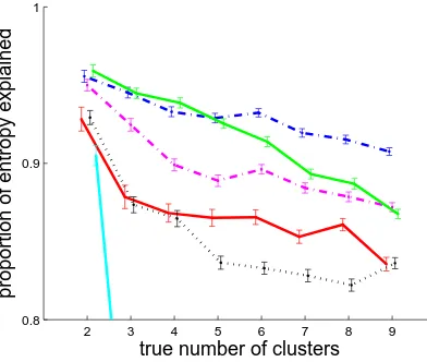
These results were consistent for between 3 and 7 true clusters. UPGMA, Ward’s method

and complete linkage performed similarly over any number of clusters; neighbour joining

formed the most poorly. We compare Euclidean distances in Figure 2.3 below because it

per-forms well and consistently between clustering algorithms. Results for all distance metrics can

be seen in Figure A.13. No single distance metric outperformed all others for any algorithm,

(44)

2 3 4 5 6 7 8 9 0.4

0.5 0.6 0.7 0.8 0.9 1

proportion with correct number of clusters

Figure 2.3: Performance of each clustering algorithm with Euclidean distance on synthetic datasets of 500 abundance profiles with 2 to 9 true clusters. Each clustering algorithm gave from 2 to 12 clusters for each dataset. The optimal number of clusters was found determined using the technique of Calinski and Harabasz (1974). The proportion of trials identifying the correct number of clusters is plotted against the number of synthetic clusters in the dataset. PE Values for neighbour joining at 3 to 9 clusters are below 0.2. Lines are blue for K-means, green for PAM, purple for Ward’s method, red for UPGMA, black for complete linkage, and cyan for neighbour joining.

2.3.2 Clinical Data

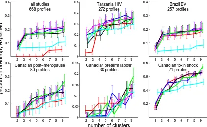
Figure 2.4 shows that K-means, PAM, Ward’s method and complete linkage performed

sim-ilarly for explaining the BV status entropy in the pooled dataset of 668 abundance profiles

from 5 studies for which information on subjects’ BV statuses were available. Neighbour

join-ing was inferior to these methods, and UPGMA clusterjoin-ing was inferior to neighbour joinjoin-ing.

Neighbour joining also performed poorly on the Brazil BV and Canadian toxin shock datasets

alone. For simplicity we have shown only the results for Euclidean distance as it was

consis-tently one of the top performing distance metrics. The results for all distance metrics are given

on Figures A.14 to A.19, although they did not differ by much. Over these datasets UPGMA

and neighbour joining performed very poorly at least once for each distance metric.

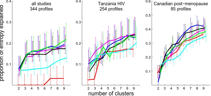
Figure 2.5 shows that UPGMA performed poorly for explaining the pH value entropy in

the pooled dataset of 344 abundance profiles from 2 studies for which information on subject’s

(45)

2.3. R 33

2 3 4 5 6 7 8 9 0.1 0.2 0.3 0.4 all studies 668 profiles

2 3 4 5 6 7 8 9 0 0.1 0.2 0.3 0.4 0.5 Tanzania HIV 272 profiles

2 3 4 5 6 7 8 9 0.1 0.2 0.3 0.4 Brazil BV 257 profiles

2 3 4 5 6 7 8 9 0.1 0.2 0.3 0.4 Canadian post−menopause 80 profiles

2 3 4 5 6 7 8 9 0 0.05 0.1 0.15 0.2 0.25

Canadian preterm labour 38 profiles

number of clusters

2 3 4 5 6 7 8 9 0.2

0.4 0.6 0.8

Canadian toxin shock 21 profiles

Figure 2.4: Performance of each clustering algorithm with Euclidean distance on clinical data with 2 to 9 clusters. The PE of the subject’s BV status is plotted against the number of a priori clusters the algorithm was asked to find. Error bars show 95% confidence intervals obtained by bootstrapping over 10,000 replicates, and are staggered on the x-axis for visibility. Lines are blue for K-means, green for PAM, purple for Ward’s method, red for UPGMA, black for complete linkage, and cyan for neighbour joining.

similarly well to each other. Neighbour joining was consistently but not significantly worse

than these four algorithms. When data from the studies were not pooled, there was insufficient

power to distinguish the performance of the algorithms. As with the BV data above we have

shown only the results for Euclidean distance here, and the results for all distance metrics are

given on Figures A.20 to A.22. The results did not differ much by distance metric. Again,

Optimal clustering techniques for metagenomic sequencing data

Scholarship@Western

Scholarship@Western

Optimal clustering techniques for metagenomic sequencing data

Optimal clustering techniques for metagenomic sequencing data

(Thesis format: Integrated Article)

by

Erik Cameron

Graduate Program in Applied Mathematics

A thesis submitted in partial fulfillment

of the requirements for the degree of

Masters of Science

The School of Graduate and Postdoctoral Studies

The University of Western Ontario

London, Ontario, Canada

c

THE UNIVERSITY OF WESTERN ONTARIO

School of Graduate and Postdoctoral Studies

CERTIFICATE OF EXAMINATION

Co-Authorship

Contents

List of Figures

List of Tables

Chapter 1

Introduction

1.1

Human Microbiota

1.2

Clustering

1.3

Our Contribution

Bibliography

Optimal clustering techniques for vaginal

microbiota

2.1

Introduction

2.1.1

Composition of Microbiota

2.1.2

Clustering

2.1.3

Our Contribution

2.2

Methods

2.2.1

Clustering

2.2.2

Synthetic Data

2.2.3

Clinical Data

2.2.4

Software

2.3

Results

2.3.1

Synthetic Data

2.3.2

Clinical Data