Assessment of vulnerability of water resources to climate variability in Mara river basin, Kenya

ASSESSMENT OF VULNERABILITY OF WATER RESOURCES

TO CLIMATE VARIABILITY IN MARA RIVER BASIN , KENYA

~~.:-\4c i .' 1 '.

BY ~ '(.) '1-r--:. -" '\ r ' -," _. - ¥ REVEL KAMAV W AITHAKA (BSc ENV, KU)

(156/l2145/09)

A Thesis Submitted in Fulfilment of the Requirements for the Degree of Master of Science (Integrated Watershed Management) of Kenyatta University

DECLARATION

This thesis is my original work and has not been presented for a degree or any other award in any other University.

Signahlfe~~

e:Kamauw:haka·

Date {CO(

Ls/'4

Department of Geography

We confirm that the candidate under our supervision carried out the work reported in this thesis

Signature~HHwHwHH~~DateJ~Jl.l~Qlyw

Department of Geography

Signature

....

H~O ~~;is~1:~:···Date...Il(~1~.L't

..

III

DEDICATION

ACKNOWLEDGEMENTS

Finally, the culmination of a journey that started with a single step and gradually developed into one mighty task. My joy and sense of fulfilment would not be complete without making mention of everyone who offered help and support, in one way or another, during the entire period of this master's study. The brevity of this acknowledgement does not in any way downplay the support I have received from anyone mentioned, or not mentioned, herein. Firstly, I am sincerely grateful to Mr and Mrs Lawrence Waithaka and East Africa office -Global Water for Sustainability (GLOWS) for their financial support in form of tuition and scholarship. to undertake this study. I thank my workmates Mr. Aron Kecha and Mr. Griffins Ochieng who gave me time to concentrate on my studies at the expense of work the office.

v

East Africa Global Water for Sustainability (GLOWS) coordinator for the efforts you made tomake sure I got the funds.

TABLE OF CONTENTS

DeeIar ati0n --- ii

De die a ti0n --- iii

A ckn0 WIed gem en ts --- iv

Tab Ie of Con ten ts --- vi

List of figures --- ..--- x

List of tables --- xi i

Acr 0n yms and Ab b r evia ti0ns --- xiii

A b str act --- xv CHAPTER ONE: INTRODUCTION --- 1

1.1 Background of the study 1

1.2 Statement of the problem 3

1.3 Justification of the study 3

1.4 Research questions .4

1.5 Objectives of the study .4

1.5.1 Main objective .4

1.5.2 Specific objectives 5

1.6 Significance of the study 5

l.7 Scope and limitations of the study : 5

1.8 Operational definition of terms 6

CHAPTER TWO: LITERATURE REVIEW --- 8

2.1 Introduction 8

VII

2.3 Impact of climate change and variability on water resources 9

2.4 Linking climate change and water resources 9

r:

2.5 Assessment of vulnerability and climate variability 10

2.6 Climate Variability analysis by NDVI 13

2.7 Conceptual framework 16

CHAPTER THREE: MATERIALS AND METHODS---20

3.1 Introduction 20

3.2 The study area 20

3.3 Climate of the study area 22

3.4 Socio-economic Characteristics 22

3.5 Sampling Techniques 22

3.6 Data collection and quality control 24

3.7 Data type and sets 24

3.7.1 Objective One: Hydro-meteorological data 24 3.7.2 Objective Two: Satellite images and Remote Sensing Data 26

3.7.3 Objective Three: Socio-economic data 27

3.8 Data analysis methods 28

3.8.1 Objective One: Hydro-meteorological 28

3.9.3 Objective Two: Digital image processing and analysis 31 3.8.2 Objective Three: Socio-economic data analysis 36 CHAPTER FOUR: RESULTS AND DISCUSSION ---37

4.1 Introduction 37

4.2.1 Climatic trend analysis 37 4.2.2 River flow trend analysis results 41 4.3 Objective Two: Satelite imagery analysis results .45 4.3.1 Assessment of Land use/land use change .45 4.3.2 Assessment of Normalized Difference Vegetation Index (NDVI)49 4.3.3 Mara River Basin water bodies trend from 1985 to 2010 54 4.4.1 Influence of climate variability on the socio-economic livelihoods55

4.5 Discussion of Results 77

4.5.1 Objective One: Hydro-climatic trends in the Mara river basin 77 4.5.2 Objective Two: Assessment of land use/ land use changes in the Mara

river basin 91

4.5.3 Objective Three: Assessment of the influence of climate variability on the socio-economic livelihoods in the Mara river basin 97

CHAPTER FIVE: SUMMARY OF FINDINGS, CONCLUSIONS AND

RE COMMEND A TI 0N S--- 103

5.1 Introduction 103

5.2 Summary offindings l03

5.2.1 Objective One: To examine the hydro-climatic trends in the Mara River basin 103

5.2.2 Objective Two: To examine the hydro-climatic trends interactions with land use/land use change that influence water resources vulnerability ... 106 5.2.3 Objective Three: To assess the influence of climate variability on the socio-economic livelihoods in the Mara river basin 107

IX

5.3.1 Objective One: To examine the hydro-climatic trends in the Mara River basin 108

5.3.2 Objective Two: To examine the hydro-climatic trends interactions with land use/land use change that influence water resources vulnerability ... 110 5.3.3 Objective Three: To assess the influence of climate variability on the socio-economic livelihoods in the Mara river basin 112

5.4 Recommendations 113

5.4.1 Objective one: To examine the hydro-climatic trends in the Mara River basin 113

5.4.2 Objective two: To examine the hydro-climatic trends interactions with land use/land use change that influence water resources vulnerability ... 114

5.4.3 Objective three: To assess the influence of climate variability on the socio-economic livelihoods in the Mara river basin 114

LIST OF FIGURES

Figure: 2-1 Conceptual framework for assessing climate vulnerability. Adopted and

modified from (F"ussel &Minnen, 2002) 18

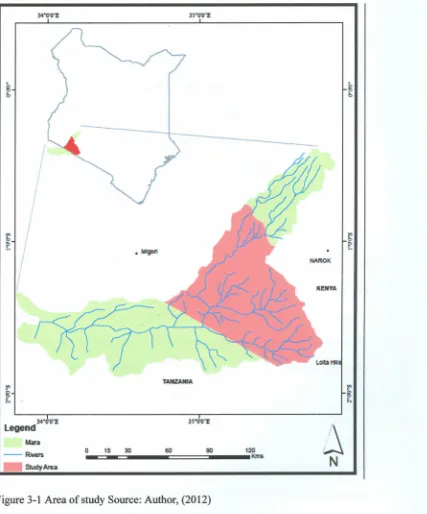
Figure 3-1 Area of study Source: Author, (2012) 21

Figure 3-2 River gauges and weather stations in the area of study. Source: Author,

(2013) 25

Figure 3-3 Image classification workflow (Source: ESRI, 2010) 32 Figure 3-4 Area of study in the context of the Landsat scenes used (Source: Glovis,

2012; WRI, 2008) 34

Figure 4-1: Maximum and Minimum temperature at Narok Station. Source: (Field

Data, 2013) 38

Figure 4-2 Average annual rainfall at Narok station. Source: (Field data, 2012)39 Figure 4-3 Average yearly rainfall at Ilkerin station. Source: (Field data, 2012)40 Figure 4-4 Monthly total average Amala RGS 1956-1995. Source: (Field data, 2012)

... 41 Figure 4-5 Total annual averages river flows for Amala RGS (1956-1995). Source:

(Field data, 2012) 42

Figure 4-6 Monthly average totals Nyangores RGS (1964-1999). Source: (Field data,

2012) 43

Figure 4-7 Total averegae flows Nyangores RGS. (Source: Field data, 2012) 44 Figure 4-8: Land use thematic maps from 1985-2010. (Source, Author 2013)46

Figure 4-9: Normalised Difference Vegetation Index (NDVI) Images (1985-2010).

(Source: Field data, 2013) 50

Figure 4-10: Normalized Difference Water Index (NDWI) images (1985-2010).

Xl

Figure 4-11: Summarised surface water trends from 1985-2010. Source (Field data,

2013) 55

Figure 4-12: Size ofland of the respondents. Source: (Field survey, 2013) 61 Figure 4-13: Type of crops grown (Source: Field survey, 2013) 63 Figure 4-14: Food deficiency months. (Source: Field survey, 2013) 64 Figure 4-15 Challenges of livestock lceeping. (Source: Field survey, 2013) 66 Figure 4-16: Causes of drought (Source: Field survey, 2013) 67 Figure 4-17: Frequency of the droughts (Source: Field survey, 2013) 68 Figure 4-18: Sources of water in the study area. (Source: Field survey, 2013)69 Figure 4-19: Challenges in water accessibility. (Source: Field survey, 2013) .71 Figure 4-20: Solutions to water accessibility and availability. (Source: Field survey,

2013) 72

Figure 4-21: Observed climate changes. (Source: Field survey, 2013) 73 Figure 4-22: Major effects of climate change on the households. (Source: (Field

survey, 2013) 74

LIST OF TABLES

Table 3-1: Satellite images used in the study 26

Table 3-2 Weather stations utilized in the study 30

Table 4-1: Summary of Land use thematic map .47

Table 4-2: Summarised household characterization 57

Table 4-3: Land utilization 61

Table 4-4: Reasons for food deficiency 64

Table 4-5: Type of livestock 65

Table 4-6: Types of water uses 69

Table 4-7: Distance travelled 70

Table 4-8: Types of sources of water 70

Table 4-9: Adherence and effectiveness ofEWS information 77 Table 4-10: Temperature and rainfall scenarios and potential effects on water

Xlll

ACRONYMS AND ABBREVIATIONS

ALRMP Arid Lands Resource Management Programme AOI Area of Interest

ASALs Arid and Semi-Arid Lands ENSO EI Nino Southern Oscillations

ESARO East and Southern Africa Regional Office ETM Enhanced Thematic Mapper

EWS Early Warning systems GCM Global Circulation Models

GIS Geographical Information Systems GPS Global Positioning Systems

IIRR International Institute for Rural Reconstruction IPCC Intergovernmental Panel on Climate Change

IR Infra-Red

KMD Kenya Meteorological Department LANDSAT Land Satellite

LULC Land Use Land Cover LVB Lake Victoria Basin

MDGs Millennium Development Goals

MK Mann Kendall

MMNR Maasai Mara National Reserve

MWI

NDVI

NDWI

NIR

RGS

SOE

SSA

TAR

TM

UNEP

UNEP

USGS

WRMA

WFP

WWF

Ministry of Water and Irrigation

Normalized Difference Vegetation Index

Normalised Difference Water Index

Near Infra-Red

River Gauging Stations

State of Environment

Sub Saharan Africa

Third Assessment Report

Thematic Mapper

United Nations Environmental Program

United Nations Environmental Programme

United States Geological Survey

Water Resources Management Authority

World Food Prograrnme

xv

ABSTRACT

Different African regions have been recognized to have climates that are among the

most variable in the world on intra-seasonal to decadal timescales. The continent is

characterized by a highly variable climate (Hulme et al.. 2001) climate change

models suggest that, in general terms, the climate of Africa will become more

variable. Although the exact nature of the changes is not known and remains debatable, there is general consensus that extreme events willmore frequent and may

get worse (Elasha, 2006). The (IPCC, 2001) report cites changes in some extreme

climate phenomena indicating that extreme events, including floods and droughts,

are becoming increasingly frequent and severe. According to (IPCC, 2001), impacts

of climate change in Africa are likely to be more severe on the continent's water

resources and food security, precipitation and insulation, length of growing seasons, water availability, carbon uptake, incidences of extreme weather events, changes in

flood risks, drought, distribution and prevalence of human diseases and plant pests. It is probable that these increased frequency of disasters results from a combination of

climatic variability, socio-economic and demographic changes.

The variability in climate particularly the changes in temperature, precipitation and

sea levels are expected to impact on availability of freshwater. This is of particular concern to Africa, where around 300 million people have no access to potable water

2

Wit & Jacek, 2006). Due to the inter-annual variability of rainfall, people are

becoming reliant on other sources like groundwater and water harvesting as their

source of freshwater. Studies by (Stutcliffe & Knott, 1987: Groove, 1996; Conway,

2002) demonstrate high levels of inter-annual variability in many river basins of

Africa. This variability is experienced mostly in dry areas (less than 800mrn of

rainfall per annum).

Global wanmng is rendering the climates of some regions dryer and all more

variable and unpredictable (Parry, 1992). For example, the arid and semi-arid of

sub-Saharan Africa (SSA) are characterizecl by limited water supply, low and highly

variable rainfall, and recurrent droughts. High temperatures and intense precipitation,

associated with achanging climate, causes increased water loss through evaporation

and run off, respectively (IRR, 2002). The rainfall is bimodal and characterised by

spatial-temporal uncertainty. Rainfall seasonality affects forage availability, livestock

production and ultimately the livelihoods of pastoralists. The 1998 El Nino

phenomenon produced an estimated five-fold increase in rainfall (G1alvin et al., 2001) the phenomenon fell between some of the worst drought years in 1997 and

1999 according to (WFP, 2000). Such extremes of climate variability make

funclamental changes to ecosystem structure and function. These in turn affect human

land-use, wildlife and livelihoods and have the potential to make these populations

more vulnerable. The Mara River, rises on the Mau escarpment in Kenya an

important water tower, is one of the most ecologically important trans-boundary river

sustainability of the nver basin, with potentially detrimental impacts on the ecosystem as a whole. This study therefore attempts to assess the vulnerability of the water resources within the basin caused by climate variability.

1.2 Statement of the problem

Climate adaptation research, while it has provided vital information in understanding climate change and variability, it has had its focus on climate change scenarios

emphasizing more on technical and infrastructural adaptive strategies to climate variability. This approach limitedly accounts for varying climates in terms of rainfall amounts, duration and temperatures especially at local levels, where adaptive and coping strategies are needed most. The Mara river basin is undergoing ecological changes that are associated with deforestation on the Mau catchment, and land tenure changes due to expansion of cash crops and settlements, among other factors. The above factors coupled with potential climatic variability, already witnessed in the East African region, have negatively impacted on water resources within the Mara river basin. This study therefore seeks to add information and knowledge on the status of the water resources and the impact of climate variability to ensure timely detection and predication of any impacts.

1.3 Justification of the study

Water resources and livelihoods particularly in Sub-Saharan Africa are highly vulnerable to year-year climate variability. To resource-limited households who

4

water scarcity remains a challenge. It is anticipated that assessment of vulnerability to climate variability would go along way to capture the multiple factors that impact on people's livelihoods especially to water sources. This study identified the Mara river basin in Kenya, a semi arid area susceptible to rainfall variability, the main social economic activity being pastoralism, tourism and both small and large-scale mechanized farming. The area depends on Mara River, swamps and seasonal rivers namely Talek, Engare Ngobit and Sand River. Given the effect of climate variability on water resource. This assessment offers a wider scope in developing strategies for efficient water resource management in thebasin, as there isneed to adapt to changes in the volume, timing and quality of water (Wigley, 2005)

1.4 Research questions

1. How are the hydro-climatic trends in the Mara river basin?

11. How does the trends interact with land use/land use change to influence vulnerability of water resources

111. How do the trends influence vulnerability of socio-economic livelihoods?

1.5 Objectives of the study

1.5.1 Main objective

1.5.2 Specific objectives

i) To examine the hydro-climatic trends in the Mara river basin

ii) To examine the hydro-climatic trends interactions with land use/land use

change that influence water resources vulnerability.

iii) To assess the influence of climate variability on the socio-economic

livelihoods in the Mara river basin.

1.6 Significance of the study

Climate variability and water resources management are significant global issues

with regional, national and local impacts. This is evident in Kenya where an

increasingly variable climate has resulted to prolonged drought and widespread

flooding. This study assesses the risks to water resources due to climate variability

and change. This is significant in policymaking and implementation especially in

water resources management, planning and design of infrastructure. It is widely

recognized that improved incorporation of current trend of climate variability would

make future adaptation easier. Water resources management is clearly linked to other

policies; hence the study aligns adaption measures across multiple water dependant

sectors.

1.7 Scope and limitations of the study

The study is based in the Mara river basin in Kenya, the middle catchment of the

6

vulnerability of water resources to climate variability within the sub-catchment. It

utilises datasets such as river flow data, temperature, and rainfall and satellite

images. The study utilizes river flow gauging stations namely Nyangores and Amala,

two weather stations namely Narok (1980-2010), and Ilkerin Integral Development

(1980-1999). Assessment of vulnerability relies heavily on data and this was the

biggest limitation scanty data on rainfall, temperature and river flow data, due to lack

of temperature data the study utili sed data of adjacent weather stations with similar

altitude e, Other limitations encountered in the field were language barrier and false

responses from respondents. However, efforts were put in place to minimise their

impact on the outcome of the study.

1.8 Operational definition of terms

Adaptation: adjustments in natural or human systems in response to actual or

expected climatic stimuli or their effects, which moderates harm or exploits

beneficial opportunities.

Climate change: Changes in the mean climate on a global scale

Climate variability: Is defined as inter-seasonal and/or inter-annual variation of the

climate within a specified geographic location.

Livelihood: The capabilities, assets and activities required for means of living.

Sensitivity: The degree to which a system IS affected, either adversely or

beneficially, by climate-related stimuli.

8

CHAPTER TWO: LITERATURE REVIEW

2.1 Introduction

This chapter reviews empirical works done by other scholars in the field of climate

variability and its effect on water resources and management. The chapter deals with

role of climate variability and the link to water resources, and inherently the

assessment of the future vulnerability and conceptual framework. It reviews studies

done specific to the basin and identifies gaps that this study attempts to fill.

2.2 Overview of climate change vulnerability

A decade of research on climate change vulnerability shows that inevitably it is the

poor and the most vulnerable who suffer the impacts of changing environmental

conditions (Adger, 2000; Downing, 2003), Vulnerability is both spatial and temporal

variable; manifested in local economic, social and cultural characteristics, as well as

the local physical conditions. The World Bank (2002) states that the linkages of

climate variability impacts to water resources are dynamic, often inter-connected,

and context-specific reflecting geographic location; economic, social, and cultural

characteristics; prioritization and concerns of individuals, households, and social

groups; as well as institutional and political constraints. This means that the

assessment of vulnerability must be made at the appropriate spatial scale for example

at sub-basin in order for it to be useful for defining the appropriate adaptation

2.3 Impact of climate change and variability on water resources

Rainfall and water resources in Africa display high levels of variability across a range of spatial and temporal scales with important consequences for the management of variability and risk in water resource systems. Studies by (Stutcliffe & Knott, 1987; Groove, 1996; Conway, 2002) demonstrate high levels of inter-annual variability in many river basins of Africa. Detailed studies of smaller size river basins in East Africa highlight changes in daily flow characteristics; for example, in Tanzania, (Valimba et al., 2008) identified the effects of human activities on the land surface and their influence on flow regimes in the Mara River Basin. He found out that the main driver of variability in river flows was of course rainfall, particularly at the scale of large river basins. Nevertheless, in spite of the large influence of rainfall fluctuations on river flow variability the response may be influenced by other factors such as changes in land cover or land use, abstraction,

hydrological characteristics (Ribot et al., 1996) argues. The actual hydrological conditions will also mediate the effects of rainfall variability; for example, lake and wetland systems may smooth and delay runoff responses according to (Adger, 2000) and semi-arid river basins with low runoff coefficients often exhibit high sensitivity to rainfall fluctuations (Nemec &Schaake, 1982).

2.4 Linking climate change and water resources

10

in the icecaps of Antarctica and Greenland leaving the remaining 30% (equal to only

0.7% of total water resources worldwide) available for consumption. From this

remaining 0.7%, roughly 87% is allocated to agricultural purposes (IPCC, 2007).

Since the Third Assessment Report (TAR) by the IPCC, there have been many

studies on trends in river flows during the 20th century at scales ranging from

catchment to global. Some of these studies have detected significant trends in some

indicators of river flow, and some have demonstrated statistically significant links

with trends in temperature or precipitation. Groundwater flow in shallow aquifers is

affected by climate variability and change through recharge processes as studied by

(Chen et al., 2002) as well as by human interventions in many locations (Petheram et

al., 2001). A variety of climatic and non-climatic processes influence flood characteristics, resulting in river floods. Floods depend on precipitation intensity,

volume, timing, antecedent conditions of rivers and their drainage basins amongst others. Kron & Berz (2007) however observed that the increase in precipitation

intensity and other observed climate changes often trigger floods, and that climate

change might already have had an impact on the intensity and frequency of floods.

2.5 Assessment of vulnerability and climate variability

The literature on vulnerability and variability assessment is very large and increasing rapidly. Brooks (2004) point out that even in the (IPCC, 2001) there is inconsistent use of the term vulnerability assessment. According to (O'Brien et al., 2002)

biophysical vulnerability, or the sensitivity of the natural environment to an exposure to a hazard; and social vulnerability, or the sensitivity of the human environment to the exposure.

Mutal et al. (2002) identified vulnerability indicators of the water resources to climate variability; they found out both natural (temperature, rainfall, evapo-transpiration) and artificial factors associated with human activities like settlements, land use/ cover change, and population increase. For the purpose of this study, the research focused on rainfall and temperature as the indicators of study due to their spatial and temporal variability. Artificial factors were used in mapping as they enhance or exacerbate the vulnerability. Kundzewicz et al. (2007) looked at impact of climate change on freshwater resources and how it has influenced water management and achievement of Millennium Development Goals (MDGs). They found out that Arid and Semi Arid Lands (ASALs) areas already experiencing water scarcity would be the most vulnerable due to decreasing water resources resulting from the decline on surface and subsurface flows. They recommend shift in water management to go beyond infrastructure development to address the problem and include forecasts, models and climate variability science in developing the water

management policies.

12

national representation does not provide any indication of how risks are distributed

across a country or region and they recommend assessment of vulnerability be

considered beyond the national scale. They point out that the assessment be done at

appropriate spatial scale in order to be useful for defining adaptation and mitigation

measures. It is against this recommendation that this study seeks to assess the

vulnerability at a local scale.

A hydro-meteorological data analysis by (Melesse et al., 2008) for the Mara river

basin showed an annual decline of 14% of rainfall in the Kaptunga forest, the river

flows of Amala and Nyangores had different hydrologic responses with Amala

having a low dry flow and a high wet flow unlike that of the Nyangores. He

concludes that high wet season and low dry season flows can be attributed to less

vegetation cover leading to low recharge in the headwaters and also flashy runoff due

to less infiltration associated with less vegetation cover but recommends further

studies on the actual cause of the flow reduction in the basin. Further research by

(Melesse et al., 2008) to model the impact of Land-cover and rainfall regime

scenarios on the flow of Mara River; used the Soil and Water Assessment Tool

(SW AT) Model to consider different input scenarios of land-cover and precipitation

pattern to estimate the changes in the hydrologic flow of the basin, The analysis

showed that a 20% reduction in rainfall translates to a46% flow reduction annually,

the model predicts a rainfall decline by 20% for the period of 2010-2030. But

according to (Ringus et al., 1996) there is contradiction with this study. His

warmer by the year 2050; annual rainfall will increase by 20% within the same period especially in the highlands while potential evapotranspiration (PET) is expected to increase in Africa region.

2.6 Climate Variability analysis by NDVI

Maps and time series of Normalized Difference Vegetation Index (NDVI) help to get insight in the changes that occur in the fractional vegetation cover pattern at a global scale. The degradation and intensification is not solely dependent on climate change. Many factors play an important role in the variation of vegetation cover; like deforestation for wood production and agricultural cropping cycles and due to forest fires and disasters. Besides this, there is anatural variation of rainfall, solar radiation and temperature depending on the seasons. Other variations occur in shorter and longer cycles, which can have decadal and multi-decadal periods. Labat (2008) analysed the long-term annual fluctuations of large river discharges by means of wavelet transforms. He concluded that the investigated rivers show interannual, 15-20-year and 28-30-year variability. Since river flow reflects rainfall and rainfall induces green vegetation, these time scales should be found in the variations of the vegetation cover as well. This can be studied by means of a NDVI time series to quantify the actual fractional vegetation cover changes caused by climate change and human activities

14

relations between NDVI and measured vegetation need to be established. NDVI is

used to study changes in the fractional ground cover. Changes in the vegetation cover

are often related to variations in seasonal weather conditions and the moisture

availability in the subsoil. Therefore relation between phonological behaviour,

climate and land use exists (Labat, 2008)

The phenology of vegetation IS influenced by temperature, moisture and soil

conditions (Andreas et al., 1984). Vegetation vanes within biannual, annual and

inter-annual periods. Variations in the vegetation cover are strongly related to the

amount and distribution of rainfall (Anyamba & Eastman, 1996). The correlation

between precipitation and NDVI was demonstrated by (Gray & Tapley, 1985;

Greegor & Norwine, 1986; Justice et al., 1986; Nicholoson et al., 1990; Tucker &

Nicholson, 1999; Eklundh & Olsson, 2003 and Martiny et al., 2006). A near linear

relation between the NDVI growing season and the rainfall was found for East Africa

and the Sahara by (Justice et al., 1986) and (Tucker & Nicholson, 1999). A strong

correlation has been found between rainfall anomalies and the onset variability of the

vegetation species in Northern Europe. Hermann et al. (2005) also found a

correlation between precipitation and vegetation cover behaviour.

Vegetation variability is strongly related to variations III surface temperature.

Buermann et al. (2003) examined the NDVI time series to relate inter-annual

variations in vegetation greenness to climate variability. They concluded that during

springtime spatial-temporal vegetation variation was strongly correlated to the

temperature variability. This variability is the main driver for the inter-annual greenness variation in the Northern Hemisphere. According to (Zhou, 2003) there is a significant relation between changes in N DVr and land surface temperature. This relation corresponds with ground-based measurements of temperature. These researches show that vegetation cover and NDVI variability are strongly related to climatic variability.

The registration of vegetation cover behaviour by satellites presents a global database for the analysis of phenology responses to climate variability. Besides regular variations, changes occur that are more permanent. According to several researches trends in vegetation cover behaviour occur. Trends were found by among others (Verhoef et al., 1996; Anyamba & Eastmen, 1996; Archer, 2004; Herman et al.,

16

Vegetation cover changes can also be directly due to anthropogenic effects. Therefore a distinction has to be made on which anomalies occur due to climatic changes and which occur due to anthropogenic influences. According to (Olsson et al., 2005) a positive trend in vegetation greenness can to a large extent be explained by an increase in rainfall, They stated that climatic influences could not explain differences entirely, which means other factors play a part in vegetation cover changes. Herman et at. (2005) made a distinction between climate driven and anthropogenic vegetation variability. They determined spatial vegetation dynamics and trends in NDVI and rainfall by means of fitting simple linear functions through the time series. Evans & Geerken (2004) did research in Syria comparing change in greenness to ground data. They found that large-scale anthropogenic increase in

livestock caused changes in vegetation cover, which were observed in satellite data. Other causes for anthropogenic vegetation cover change are for instance cutting down forest, change of land-use and diversion of water for irrigation.

2.7 Conceptual framework

Burton (1997) suggests a hierarchy of weather and climate phenomena to distinguish

single climate variables, specific weather events, and long-term processes (such as

anthropogenic climate change). Climate impacts are a function of (the change in) the

exposure of a system to climatic stimuli and of its sensitivity to these stimuli.

Climate variability and change, will affect regional climate variability in various

ways such as the frequency, intensity, and location of extreme events. Non-climatic

factors denote a wide range of properties that affect the vulnerability of a system or

society to climate change. They include ecological, economic, social, demographic,

technological, and political factors. Vulnerability is a function of the character,

magnitude, and rate of climate variation to which a system is exposed, its sensitivity,

18

_'on~6matic dril-us: demographic, socio-economic and politicaL tKhnology

t

•

..

:

:

Exposure Sensitivity

..

•.

Adaptin Capacity: Adaptation:

•

...

..

~

-

t

tourism poteatial, sector refollDS,water

infonnation harvesliDg, groUDd

diswminalion, <II ~ water use, water Impact: fuequency, intensity and umastructure, umastructure,efficient location of ex1mne eveuts (floods and dn-ersificatioo of &nniDgpractises RCUIIeDtdroughts) income,education and

fcmnal employment

Impact .o\n~·sis:trmd analysis for

'" climate parametas (ninfall and

tempeJature), LULC change trmds, NnVI analysis.

t

"

YulnuabiJity of miter nsources: ~ riwr flows, iDcreased e\'lporation, seasonalityof rivers,aosion and sedjmentalion,floods and low dIyflows.

I

I

I

I

Figure: 2-1 Conceptual framework for assessing climate vulnerability. Adopted and

modified from (F"ussel&Minnen,2002)

In this conceptualization, the vulnerability of a system to climate change includes

both an external dimension, which is represented by its exposure to climate

variations, and aninternaldimension,which comprises its sensitivity to them and its

adaptive capacity (Bohle et al., 1994). Mitigation and adaptation adjustments can

adaptation. In this conceptual framework we combine adaptation measures that are

targeted directly at the vulnerability of water resources and those that affect non

-climatic factors influencing the water resources. The adaptive capacity of the water resources determines its potential to reduce adverse effects of climate variability and change. As a result, adaptive capacity and vulnerability are negatively correlated. Non-climatic factors clearly affect the adaptive capacity of the water resources. Determinants of adaptive capacity in social systems comprise economic resources,

technology, information, skills, infrastructure, institutions, and equity (Smit &

I

Pilifosova, 2001; Yohe &Tol, 2002). Non-climatic driving forces often influence the

adaptive capacity of a system or social set up such as demographic, economic,

socio-political, and technological. Thus, vulnerability is understood as a function of three components: exposure, sensitivity and adaptive capacity, which are influenced by a

range of biophysical and socio-economic factors according to (Tiwari & Dinar,

2003). It is generally assumed to be more efficient to develop response strategies that

reduce the vulnerability of water resources in the Mara river basin to multiple stressors simultaneously than to formulate independent adaptation strategies for each

20

CHAPTER THREE: MATERIALS AND METHODS

3.1 Introduction.

This chapter introduces the area of study, climatic and socioeconomic activities of

the area. It further presents the sampling procedure, data sets and type, data

collection and data analysis methods. This is represented through maps, satellite images, thessian polygons and equations.

3.2 The study area

This study was carried out in the Mara River basin, between 0045'0"S and 34045'0"E in and between 200'0"S and 35°45'0"E. The figure 3:1 below represents the area of

NAROK

KENYA

j

N

I

I

I

I

I

• YgDfI

(

.H"O'O"E Legend

Mara -- Rivers

StudyAlea

o ~ ~ ~ ~ m

•••

-=~••

-=~ ••••-======-••••••

~

22

3.3 Climate of the study area

The climate vanes greatly with altitude; the rainfall is generally greatest on the

highlands of the basin with a mean annual value of 1400 mm year and lowest in the lowlands with a mean value of 600 mrn year (NEMA, 2010). The rainfall is bimodal expected during the months of April to May and' September and October.

Temperatures vary with altitude, but the mean annual temperature is 25°C.

3.4 Socio-economic Characteristics

About 62% of the households are smallholder farmers (Aboud et al., 2002) with livestock rearing being the second dominant activity. Tourism and wildlife are important economic activities as exemplified by the Maasai Mara Game Reserve on the Kenyan side and the Serengeti National park on the Tanzanian side (Mutie et al., 2006). These economic activities largely depend on adequate rainfall and water supply to maintain the livelihoods and ecosystem integrity.

3.5 Sampling Techniques

The Mara River Basin was selected because the two main rivers Nyangores and

The study applied mixture of sampling techniques guided by the objectives. Objective one and two applied purposive sampling while, objective on household survey applied random sampling with a total number of households being 9,500 (I<NBS, 2009). The sample size of the study was based on the total number of households in the sub-catchment, and was calculated using the following formula (Equation 1) that was adopted from (Yamane, 1967) cited in (Glenn, 1992). This formula is best placed for qualitative studies like for the case of this study.

N

n = 2 ---Equation: 3-1

1+N(O::)

Where:

n= is the sample size

N= is the total number of households in the catclunent

a =is the level of precision and/or margin oferror set at

i

The sample size computed by the formula is 98.6 (approximately 99). An additional

24

constitute the majority In the population are also presented proportionately (Mugenda, 2008)

3.6 Data collection and quality control

During the research there were challenges of data collection, such limitations in availability of good field data sets. Though it was impractical to collect comprehensive data on all hydrological variables at time-scales appropriate to catchment-scale processes, efforts were made to make use of available for the purposes of this stud)'. Yet even with these difficulties, such data was vital in order to understand catchment behaviour and response toclimate variability and change. Data used in this research was collected from various institutions and agencies while some were downloaded various research institutions. These included hydro-meteorological data, land cover, digital elevation model (DEM), and satellite imagery. Quality control was done by use of graphical, statistical and ground-truthing methods.

3.7 Data type and sets

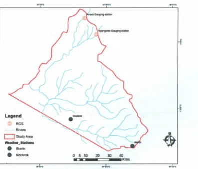
3.7.1 Objective One: Hydro-meteorological data

temperature and rainfall unlike other stations, which had only rainfall. The

temperature data from Narok Station was presumed to represent the average basin

temperature for the purposes of this study. The river flow data was acquired for

Nyangores (ILA03) (1980-2008) and Amala (lLB02) (1980-2007). The stream flow

data utilized the velocity area method to determine the volumetric stream conveyance

averages. The projection was determined based on the trends to adequately cover the

study duration.

Legend

@RGS

-- Rivers

CJ

Weather_Stations ••• erin

• Keekrdl

o

•• Kms

Figure 3-2 River gauges and weather stations in the area of study. Source: Author,

26

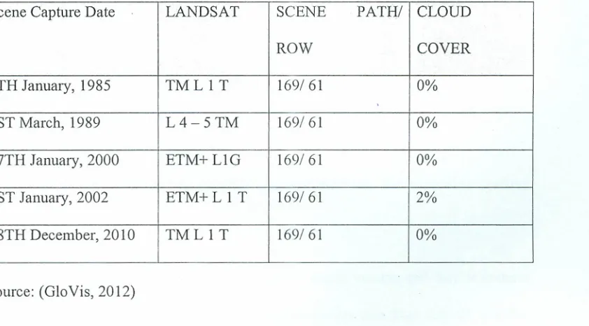
3.7.2 Objective Two: Satellite images and Remote Sensing Data

Varied categories of data were collected. Secondary data included LANDSAT

satellite images which were obtained mainly from Global Visualization website of

the United States Geological Survey (USGS). The satellite images were used to

generate false image, NDVI and NDWI images of the study area for the years 1985,

1989,2000,2002 and 2010. The images utilized in the study are summarized in the

table below.

Table 3-1: Satellite images used in the study

Scene Capture Date LANDSAT SCENE PATH/ CLOUD

ROW COVER

9TH January, 1985 TML 1 T 169/61 0%

1ST March, 1989 L4-5TM 169/61 0%

27TH January, 2000 ETM+L1G 169/61 0%

1ST January, 2002 ETM+L 1 T 169/ 61 2%

18TH December, 2010 TML 1 T 169/ 61 0%

Source: (GloVis, 2012)

Other GIS data utilized in the study were obtained from the World Resource Institute

(WRI) website. This provided the basis from which shape files of the Area ofInterest

(AOI) were generated. The Landsat satellite images for the study duration were

sampled based on their clarity, quality and equally important their availability. This

reliability of NDVI and NDWI analysis, the image dates were concentrated almost at

the same time of the year for the sampled years. Image processing and classification

utilized field knowledge, observation, ground truthing and use of GPS control points

to ensure high thematic output maps' accuracy.

3.7.3 Objective Three: Socio-economic data

The study further reviewed the understanding on vulnerability of water resources to

climate variability on shocks or risks to which households are exposed. To determine

this vulnerability, risk factors, the data was obtained using variables such

i) Socio-economic and demographic characteristics (Age, Gender, level of

education, main occupation, length of stay atstudy area, type ofhousing)

ii) Resource ownership and utilization (size, utilization, type of food crops)

iii) Water resource (access and availability)

iv) Climatic changes (noticeable seasonal changes, early warning systems

and effects)

Primary data was collected using a structured questionnaire and key informant

interviews. A structured questionnaire was used to gather data from the 104 sampled

households. Key informant interviews with 13 relevant key persons in the area

(including water department and environment office at the district and water resource

users at the local levels, opinion leaders and community groups) were used to collect

data and at the same time to complement and/or give more detailed information

28

3.8 Data analysis methods

The study applied various analysis methods to achieve the objectives of the study as elaborated below.

3.8.1 Objective One: Hydro-meteorological

Hydro-meteorological time senes almost always exhibit seasonality due to the periodicity of the weather. This seasonality anses from seasonal variations of precipitation volume and evapo-transpiration. Such kind of data requires require trend analysis that incorporates the seasonal component hence the use of trend analysis methods in this study. Simple linear regression (Y) is one of the most useful parametric models to detect trends was used in this study.

The model for Y can be described by the equation below:

Y = aX

+

Where,

X=time (year),

a=slope coefficients;

b=least-square estimates of the intercept.

interpretation is that it is entirely reasonable to interpret there is a change occurring over time. The sign of the slope defines the direction of the trend of the variable: increasing if the sign is positive, and decreasing if the sign is negative.

3.8.1.1 Determining river flow rates

30

The formula is as follows

Q

=

*

Where: Q

=

v

A = Cross sectional area of the stream profile defined by the river ?

transect (111-)

3.8.1.2 Determining the climatic trends

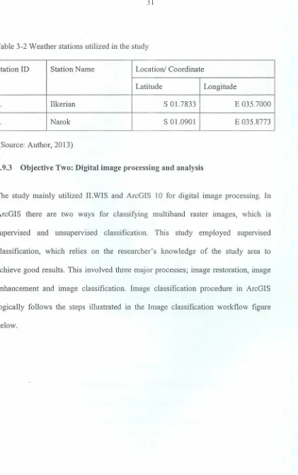
Table 3-2 Weather stations utilized in the study

Station ID Station Name Location! Coordinate

Latitude Longitude

1. _{Ilkerian SOl.7833 E 035.7000}

2. Narok S 0l.0901 E 035.8773

(Source: Author, 2013)

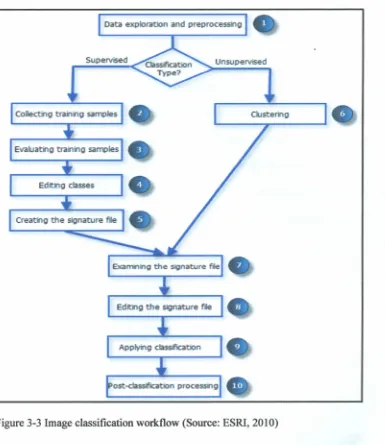
3.9.3 Objective Two: Digital image processing and analysis

The study mainly utilized IL WIS and ArcGIS 10 for digital image processing. In

ArcGIS there are two ways for classifying multiband raster images, which is

supervised and unsupervised classification. This study employed supervised

classification, which relies on the researcher's knowledge of the study area to

achieve good results. This involved three major processes; image restoration, image

enhancement and image classification. Image classification procedure in ArcGIS

logically follows the steps illustrated in the Image classification workflow figure

32

Data exploratiOn and preprocessilg

Supervised _Unsupervised

Figure 3-3 Image classification workflow (Source: ESRI, 2010)

The steps can be summarized as:

i. Display three band composite image

ii. Choose representative training samples for the desired classes

lll. Generate, manage and evaluate signature file

v. Colour code and show the classified image

To ensure high accuracy level, images were subjected to further processing to

remove noises and isolated regions for better output quality; also known as

post-classification tasks. Post classification involved: Filtering, smoothing and clumping,

and generalizing output maps. To assess the truthfulness of the classified thematic

maps; this research utilized the error matrix method for accuracy assessment (also

called covariance, correlation or confusion matrix) to ensure the accuracy level of

image processing system in correctly identifying selected classes.

To assess the distribution and healthiness of vegetation cover, NDVI computation

was used. NDVI function was ideal in determining vegetation change, an indicator

water resources vulnerability and availability. As indicated above, the path! ram of

the images utilized are 169/ 61 in which the area of interest lies as illustrated below.

34

34°4O'0"E 3S°0'0"E 3S020'0"E 3S044T0"E 36°O'o"E 36"2O'O"E

Legend _2°20'0"S

[::J

RGB Bands

t

11III

11III

11III

3·0·0·S

-

-

0 20 40 80 120 160

Figure 3-4 Area of study in the contextofthe Landsat scenes used (Source: Glovis,

2012; WRI, 2008)

NDVI uses the intensity discrepancy of bands 3 and 4, to compute the bustle of

vegetation symbolized as:

NDVI= (NIR-RED).

Where RED and NIR represent the spectral reflectance value recorded in the red and

near-infrared (NIR) ranges in the electromagnetic spectrum respectively. NDVI

values range between -1 to +1, but vegetation has NDVI values of between 0.1 and

0.7 (Roettger, 2007). The higher the NDVI the higher the fraction of live green

vegetation present in the area. Landsat band 4 (0.77 - 0.90 urn) measures the

reflectance in NIR region and Band 3 (0.63 - 0.69 urn) measures the reflectance in

Red region. ArcOIS generates the output using the following formula: NDVI =

((IR-R)/(IR+R))* 100+ 100. This results in avalue in range of 0 - 200 and fit within an8

-bit structure, these are the zeros and ones that computer space uses to write value to

each grid cell of an image. The bulk of the LAN DSA T images utilized were captured

by Thematic Mapper (TM), Enhanced Thematic Mapper (ETM) and Enhanced

Thematic Mapper Plus (ETM+) sensors mounded on Landsat 4-7. From the images,

the healthiness and intensity of vegetation cover is computed, this capacity provided

for in the calculate geometry command. The 151 order classes based on physical

characteristics of the land cover were used. The classes are forest land, barren land,

water, tundra, agricultural land, built-up land, range land and wetland (Anderson, et

al., 1976) as applicable. Trend analysis was especially conducted based on the

variation in vegetation cover change and surface water coverage trends in relation to

the area's water balance.

NDVI utilizes the chlorophyll present in plants leaves. Chlorophyll absorbs more

energy at~0.45 ~L(micron) (blue) and also marginally light at ~O.65 ~L(red), while it

36

accounts for the green colour of most plants. NDVI utilizes this distinctive spectral behaviour of chlorophyll for visualization, depicted by the difference between calculated solar reflection from a satellite band very sensitive to chlorophyll (~0.65

~L)and a band in the red part of the visible spectrum (~O.65 ~L).Values below 0.15 are not shown in NDVI but instead are replaced by natural colour imagery that represents barren land (Wu, Niu, Tang, &Huang, 2008).

3.8.2 Objective Three: Socio-economic data analysis

The data analysis compromised both qualitative and quantitative techniques. Data

screens were prepared using SPSS version 19, then the corded data was keyed on the software for descriptive analysis. The descriptive analysis gives frequencies and proportions. This study used bivariate analysis techniques to assess to the

relationships between independent and dependant variables: cross tabulations were used to generate the rows and column percentages for the interactions between the

CHAPTER FOUR: RESULTS AND DISCUSSION

4.1 Introduction

This chapter presents the results and discusses the findings of the study. The results

are divided into two climatic data and land cover data analysis. The findings are

presented in form of graphs, tables and satellite images. Photographs taken in the

field also formed part of data presentation. Interpretation was done in reference to the

stated study objectives and hypothesis.

4.2 Objective One: Hydro-climatic trends results

To understand the study objective, this study sought to analyse the nature and trends

of temperature and rainfall and river flow in the middle catchment of the Mara River

Basin. Rainfall and temperature were presented in graphs and weather maps. River

flow was analysed and presented in graphs monthly and yearly totals.

4.2.1 Climatic trend analysis

The figures below provide a synthesized aggregate summary of the Mara Basin

monthly and annual rainfall from Ilkerian and Narok station. The data span varied as

38

30

'"

~w

_•

---!i

i

f

~

---...

Y-4'0107~.14,1_

---R'%0.03203

5

1980 1985 1990 1995 2000 2005 2010

-maxfemp -Mill Temp -Unear (maxTempi -Unear(M.nTempl

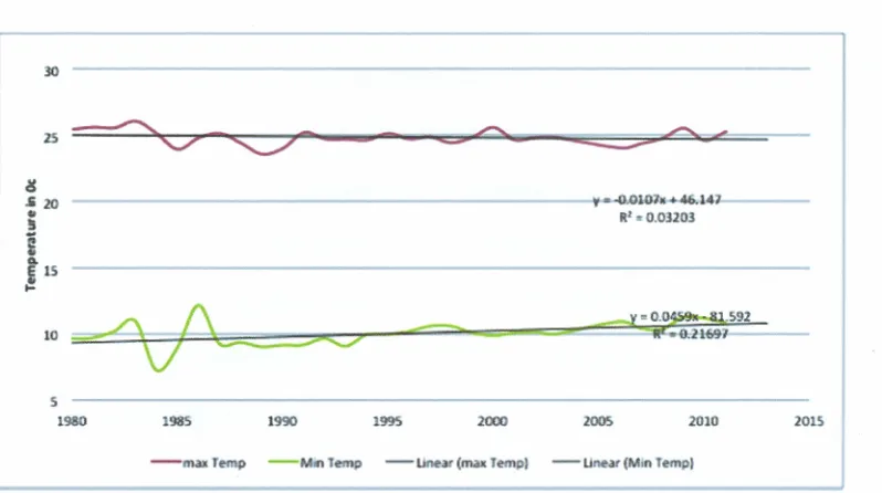
Figure 4-1: Maximum and Minimum temperature at Narok Station. Source: (Field

Data, 2013)

Figure 4: 1 shows a slight increase in minimum temperature at the Narok Station. The

R2 is given as 0.21697 indicating that the temperature has increased with an average

of O.2°C every year and therefore projected to increase with the same margin. Where Y equation shows a negative, the R2 denotes a decreasing trend and vice versa when

the equation shows positive. Thus the maximum temperature has anR2 of -0.033 this

shows a decreasing trend. These results represent close findings by (Odada &Olago,

2002; IPCC, 2007) which indicated that the air temperature in East Africa would

increase by 5°C by 2050, while us rainfall will increase by 20%. The increase in

temperature has a significant effect on water resources due to evaporation increase,

Increased temperature will lead to loss soil moisture a significant in agriculture and

determining the NDVI of the vegetation. The IPCC (2007) report summarizes the

effect of such temperature increase by stating that warmer temperatures will lead to a

more vigorous hydrological cycle. This translates into prospects for more severe

droughts and/or floods in some places and less severe droughts and/or floods in other

places. IPCC models indicate an increase in precipitation intensity, suggesting a

possibility for more extreme rainfall events (IPCC, 2007) thus making water

resources inherently vulnerable especially in arid environments like the area of study

which are characterized by non linear relationships between rainfall and run off.

1000

5

!

3

=

5600

~ ~500

e

I»

~ 400

300

~---1980 1985 1990 1995 2000 2005

Years

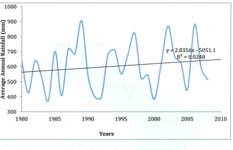
Figure 4-2 Average annual rainfall at Narok station. Source: (Field data, 2012)

Figure 4:2 representing Narok weather station shows an increasing rainfall trend. The

40

average rate of change in the hydrologic characteristic. If the slope is statistically

significantly different from zero, the interpretation is that it is entirely reasonable to

interpret there is a change occurring over time. The sign of the slope defines the

direction of the trend of the variable: increasing if the sign is positive, and decreasing

if the sign is negative. Thus the R2 is given as 0.02 indicating a linear increase of

rainfall annually by about 0.02mm of rainfall. The graph shows peak years of 1989,

1997,2002 and 2006. The results show a cyclic trend at first then the period of the

cyclic reduces to about 5years. The years 1984, 1986, 1991, 1992, 2000 and 2005

shows low rainfall amounts. This low rainfall below 400mm annually could be

attributed to the drought. These results shows much inter annual variability as

compared to other stations

"'"

S 500

!

~ 400 ~

.

5

200 800

700

600

100

o

+---~---~---_.---__,

1980 1985 1990 1995 2000

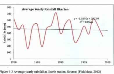
Figure 4:3 represents Ilkerin weather station data, the data shows inter annual

variability, the rainfall between consecutive rainfallvary greately. The Y equation is

negative indicating a decreasing a gradient of 0.002 as shown by the R2. R2 shows a

negative linear equation indicating that there 0.002 mm annual decrease of rainfall.

The station is located on the lower edge of the basin thats exhibits higher aridity

characteristics as compared to other stations.

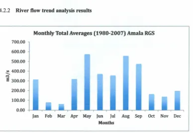
4.2.2 River flow trend analysis results

Monthly Total Averages (1980-2007) Amala RGS

700.00

600.00

500.00

~ 400.00 M

e

200.00

100.00

0.00

Ian Feb Mar Apr May [un Jul Aug Sep Oct Nov Dee

Months

Figure 4-4 Monthly total average Amala RGS 1956-1995. Source: (Field data,2012)

Figure 4:4 shows the monthly average totals; May has the highest flow above

572m3/s with March having the low flow of 61m3/s. The graph shows seasonal river

flow with high flows experienced during the months of April to September and

relative flows during October,November, February and March. The river flow can

42

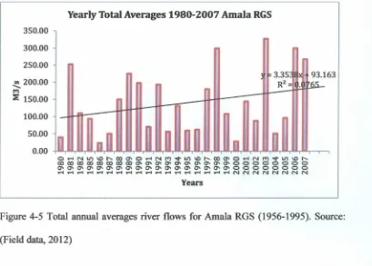
Yearly Total Averages 1980-2007 Amala RGS

350.00

300.00

250.00

~ 200.00

M

:;: 150.00

100.00

50.00

0.00

Years

Figure 4-5 Total annual averages river flows for Amala RGS (1956-1995). Source:

(Field data,2012)

Figure 4:5 shows the annual average river flow at Amala RGS. The flows are

characterized by cyclic trends of high peaks followed by low flows. The nature of

these trends have great impact on the use water resources, when there are low flows

like during the years 1980, 1986and 2000 any over abstraction may lead to flows

beyond the reserve flows. These low flows coincide with droughts and famine. High

flows are associated with favourable rainfall seasons, the area experiences flash

floods mostly by the seasonal rivers as opposed to permanent rivers such as

500.00

450.00

400.00

350.00

300.00

In

;;;-Z50.00

:e:

200.00

150.00

100.00

50.00

0.00

Monthly Total averages (1980-2008)

[an Feb Mar Apr May [un [ul Aug Sep Oct Nov Dee

Months

Figure 4-6 Monthly average totals Nyangores RGS (1964-1999). Source: (Field

data,2012)

Figure 4:6 shows the monthly averages at Nyangores river, the results indicate

different river flows as compared to Figure 4:4 the monthlyaverages of Amala RGS.

The river shows higher river flows with the month of May having the highest flow of

above 450m3/s, the flows remain above 30Om3/s and rise again to above 400m3/s in

September and drop gradually to March and then start to rise again in April. These

flows have implications in water resources in that Nyangores shows higher river

44

Yearly Total Averages-Nyangores RGS

200.00 180.00 160.00 140.00 ~20.00 ~OO.OO ::E80.00

60.00 40.00 20.00

0.00 -tU,.u.,,.u.,.u,.U-rI..y..y..YJ~...u,,.u.,.u,.U-rI..y..y..YJ~...u,,.u.,.u,.U-rI..y..y..YJ'r--r---1

y=1.3 9x+91.73 451

Figure 4-7 Total averegae flows Nyangores RGS.(Source: Field data,2012)

Figure 4:7 shows the annual average river flows. Thetrend line shows cyclic nature

with high peaks and low flows. The high peaks fall between years 1970, 1978

followed by a relative flow above 120m3/s for years 1982, 1988, 1989, and 1992.

Low flows of below 60m3

I

s

and 2000.The high flows concide withwithhigh rainfall recorded as shown in figure

4-5. There is attenuation of the river flow with the time between the onset of the rains

and the peak flow getting smaller over the years. Since rainfall and land surface

conditions are the factors that affect river flow,and since the rainfall pattern has not

changed much, the basin surface conditions are left to bethe major factor affecting

4.3 Objective Two: Satelite imagery analysis results

4.3.1 Assessment ofLand use/ land use change

The study analysed satellite imagery of inter-data variations in land-use/ land-cover

(LULC) changes between 1985 and 2010. Based on the basin's climatic conditions

which influence the region's agro-climatic zone, anthropogenic activities, flora and

fauna, and water distribution the Landsat images were classified into four land-use

classes namely: forest! shrub land, crop land/ range lands, water and bare land. As

indicated below, the basin's LULC phenomena have substantially varied between

'

...

...

,..•.•

,'un

,..•..•

•••••OHI

~

,..•...• _{••••••••}

~

LqtOHI ~·{"",...;.,I~I.,.-s

;. . ~. ,."'"

0

--_

0

--_

IF__

N

1--

-

--.-

t

.

-

t

0-""",,"

_1:

_'

_-"

_,

_,-

-

t

1- ,..,.. _1-

-

-

I-

__

.

-0 10 20 40 60 _{0 10 20 40 60}

0 10 20 40 eo eo

"

.

•..•

-,

",,"M )!I'IWt ,Ijj'rt

,..,....

0"'-_

.

.

-

.-10 to 20 "0 10 .~

I'IC'f'1

.

t

I.••••••

0

--_

.-- N

0

-_

A

.

-• - KIomtItr.

I

o W 20 40 60 60

n

,...,

.,...

...•...•

.

...

.

.

...

•

a b c

Figure 4-8: Land use thematic maps from 1985-2010. (Source, Author 2013)

d

..

.

Figures 4:8 above shows the land use thematic map indicating areas of forest/ shrub

land, river streams indicated as blue and bare lands indicated in shades of grey. The

dense green colour indicates forests and shrub lands, the light green indicating

farmlands/rangelands, blue colour indicating water bodies and grey shades indicating

bare land. Figure 4:8a indicates the land use thematic map of 1985 showing patches

of dense forests and quite significant percentage of bare land. Figure 4:8b indicates

the land use of 1989 an improvement with reduced bare land increased rangelands

and less dense forests. Figure 4:8c a rather decreased shade of green, indicating

stressed vegetation starved off water with central region showing patches of bare

land. Figure 4:8d indicates the dense green shades, this was after the rains where the

ecological phenology characteristic of grass allows it to sprout within a short time

after the rains. However the areas bordering Loita Hills and Nguruman Escarpments

continues to indicate dense forests on the southeast edge of the map. Figure 4:8e

showed increased aridity as indicated by an increased in bare land especially in new

locations earlier not noted in the previous analysis. There is quite a significant

48

Table 4-1: Summary of Land use thematic map

Land-use Area in square kilo metres (krn") Change %

class 1985 1989 2000 2002 2010

Forest! 1,378.4 986 879.5 2587.6 849.3 -529.10 -38.39

Shrub-land

Crop-land/ 4,122.6 5,126.7 5,134.7 3510.8 5,314.5 l.191.90 28.91

Range-land

Water 17.7 14.4 12.8 11.9 _15.8 -1.90 -10.73

Bare-land 1114.4 505.9 606.1 522.8 453.5 -660.90 -59.31

(Source: Field data, 2013)

The table 4: 1 above surnmanzes the inter-data variations in land-use! land-cover

(LULC) changes between 1985 and 2010. Based on the basin's climatic conditions

which influence the region's agro-climatic zone, anthropogenic activities, flora and

fauna, and water distribution the Landsat images were classified into four land-use

classes namely: forest/ shrub land, crop land/ range lands, water and bare land. The

basin's LULC phenomena have substantially varied between 1985 and 2010. Water

resource availability as depicted through the aerial extent of water distribution

indicates that water vulnerability is on the increase in the duration of 25 years (1985

- 2010).

Forest! shrubland decreased from 1378.4km2 to 986 km2due to decreased rainfall in

monthly low flow of 5.3m3/s during the same month the rainfall stations did not

record rainfall while Narok station recorded 15.3mm. In 2002 the surface coverage

increased tremendously to 2587.5km2 the same month and year recorded river flows

of 1.96m3/s and 1.32m3/s in Nyangores and Amala respectively. This difference can

be explained due to the phenology of the vegetation which turn lavish green with

little rainfall

4.3.2 Assessment of Normalized Difference Vegetation Index (NDVI)

NDVI represents the greenness of vegetation with deep green indicating dense forest

with healthy vegetation and red colour indicating no vegetation. Maps and time

series of NDvr help to get insight in the changes that occur in the fractional

vegetation cover pattern. Since rainfall induces green vegetation, time series analysis

should indicate the variations of the vegetation cover as well. To get a correct

variations of the vegetation behaviour NDVI must be established. Changes in the

vegetation cover are often related to variations in seasonal weather conditions and

the moisture availability in the subsoil. This is the relation between phonological

behaviour, climate and land use which the study sought to assess. Temperature,

moisture and soil conditions influence the phenology, thus vegetation varies

biannual, annual and inter-annual periods. Variations in the vegetation cover are

LEG!.,')) • Nco-VIgClIliOll

.V~

• 15 30 eo 11)-"

Jt'n"t u'lm W,IfII'I W~W'6 N

t

ru•••

'

.

...

wtm

• 15 30 eo

11)-'''.!fill

"'" I1'lm

•...••

~ " to 1\ 15 30 eo WJKIt:!tWttMt

"

...

,

.

...

I'I~

...••

"""" WI," H'JfI"I'.

Uct'l'D .l\oool·••• .VtllQ1ioD

' . ,,..,

II. 11. • C",....

e

a b c d

Generally during NDVI analysis the green colour denotes healthy vegetation while red colour no vegetation, NDVI cannot detect any chlorophyll on the vegetation,

hence the red colour. Figure 4:9a shows the NDVI for year 1985 with mixed

indications of dark green parches around the Lolgorian forest reserve and the eastern part in Loita Hills. The reddish yellow denotes no vegetation. When compared to the year 1989 in figure 4:9b the dark green colour intensifies indicating that by the time

of satellite image the vegetation was healthy. Figure 4:9c shows NDVI image of the year 2000 indicates the worst vegetation quality and distribution this is echoed bythe land-use thematic values. During this year the basins surface water resources constituted only about 12.8 Ian:! of the basin's aerial coverage of about 6633 km2as shown in Table 4:1.This is approximately 0.2% of the basins land mass. This ahuge decrease compared to 17.7% and 14.4 % of the previous image analysis of figure 4:8a and Figure 4:8b. The red colour on the image could be attributed to the 2002

drought that affected the whole country and study area as well. There is an increase in cropland/range land from 62% to 77% this is probably attributed to cropland

devastation by drought and famine. In figure 4:9d shows pale red and yellow, this indicates no vegetation. When compared with land use thematic image in figure 4:8d

there was an increase in cropland and rangeland, due to the characteristics of phenology of grass, when grass dries it denotes vegetation devoid of enough

52

cover with water bodies surface area mcreasing by 4km2 as compared from the

a

N

i

_i

t

N

!

c

Figure 4-10: Normalized Difference Water Index (NDWI) images (1985-2010). Source (Field data, 2013)