Accelerated Imaging Techniques for Chemical Shift Magnetic Resonance Imaging

(1)

Supervisor

Charles McKenzie

The University of Western Ontario Graduate Program in Physics

A thesis submitted in partial fulfillment of the requirements for the degree in Doctor of Philosophy

Follow this and additional works at: https://ir.lib.uwo.ca/etd

Part of the Other Physics Commons

Recommended Citation Recommended Citation

Wiens, Curtis N., "Accelerated Imaging Techniques for Chemical Shift Magnetic Resonance Imaging" (2013). Electronic Thesis and Dissertation Repository. 1465.

https://ir.lib.uwo.ca/etd/1465

This Dissertation/Thesis is brought to you for free and open access by Scholarship@Western. It has been accepted for inclusion in Electronic Thesis and Dissertation Repository by an authorized administrator of

(2)

by

Curtis N. Wiens

Graduate Program in Physics

A thesis submitted in partial fulfillment of the requirements for the degree of

Doctor of Philosophy

The School of Graduate and Postdoctoral Studies The University of Western Ontario

London, Ontario, Canada

(3)

ii

chemical shift imaging using compressed sensing and/or parallel imaging for two applications: water-fat separation and metabolic imaging of hyperpolarized [1-13C] pyruvate.

Spatially varying noise in parallel imaging reconstructions makes measurements of the signal to noise ratio, a commonly used metric for image for image quality, difficult. Existing approaches have limitations: they are not applicable to all reconstructions, require significant computation time, or rely on repeated image acquisitions. A signal to noise ratio estimation technique is proposed that does not exhibit these limitations.

Water-fat imaging of highly undersampled datasets from the liver, calf, knee, and abdominal cavity are demonstrated using a customized IDEAL-SPGR pulse sequence and an integrated compressed sensing, parallel imaging, water-fat reconstruction. This method offers image quality comparable to fully sampled reference images for a range of acceleration factors. At high acceleration factors, this method offers improved image quality when compared to the current standard of parallel imaging.

Accelerated metabolic imaging of hyperpolarized [1-13_{C] pyruvate and its metabolic}

by-products lactate, alanine, and bicarbonate is demonstrated using an integrated compressed sensing, metabolite separation reconstruction. Phantoms are used to validate this technique while retrospectively and prospectively accelerated 3D in vivo datasets are used to demonstrate feasibility. An alternative approach to accelerated metabolic imaging is demonstrated using high performance magnetic field gradient set.

(4)

iii

imaging. An approach to SNR assessment for parallel imaging reconstruction is proposed and approaches to accelerated chemical shift imaging are described for applications in water-fat imaging and metabolic imaging of hyperpolarized [1-13C] pyruvate.

Keywords

(5)

iv

method of SNR measurements that the proposed method was compared to. Jacob Willig-Onwuachi and Charles McKenzie provided advice regarding experimental validations and assisted in the preparations of the manuscript. In vivo datasets were acquired by Cyndi Harper Little.

The work in chapter 3 entitled “R2*-corrected Water-Fat Imaging using Compressed Sensing

and Parallel Imaging” is published in the journal Magnetic Resonance in Medicine and is co-authored by Curtis Wiens, Colin McCurdy, Jacob Willig-Onwuachi and Charles McKenzie. Curtis Wiens was responsible for the implementation of the proposed image reconstruction, the implementation of the MRI pulse sequence used to validate the proposed image

reconstruction, and the writing of the manuscript. Colin McCurdy assisted in the

development of the pulse sequence. Jacob Willig-Onwuachi and Charles McKenzie provided advice regarding experimental validations of the image reconstruction and pulse sequence. In addition, they assisted in the preparations of the manuscript. In vivo data were acquired by Trevor Szekeres.

The work in chapter 4 entitled “Accelerated 13_{C Chemical Shift Imaging of Hyperpolarized}

Pyruvate” is in preparation for submittion to the journal Magnetic Resonance in Medicine and is co-authored by Curtis Wiens, Lanette Friesen-Waldner, Trevor Wade, Kevin Sinclair, and Charles McKenzie. Curtis Wiens was responsible for the implementation of the

proposed image reconstruction, the implementation of the MRI pulse sequence, data

(6)

v

(7)

vi

on it. It wasn’t always clear what direction this project would go but I learned a lot along the way.

Secondly, I’d like to thank Jacob Willig-Onwuachi. Jake, you were like a 2nd supervisor to me. Your attention to detail makes you great to work with. Throughout this PhD, I always got you involved in my work. It was clear very early on, that your involvement always resulted in better manuscripts and a better understanding of my work.

The task of familiarizing oneself with GE’s pulse sequence programming language EPIC is daunting. Trevor Wade, Ann Shimakawa, and Alexei Ouriadov played instrumental roles in the completion process. Trevor, thank you for teaching me the fundamentals of pulse sequence programming and always making time to answer my questions. Your first email regarding EPIC programming entitled “You want to program in EPIC? Run while you still can” has been viewed many times throughout the course of this PhD. Ann, thank you for your assistance with the IDEAL-IQ pulse sequence. Whenever I got stuck implementing one of my crazy ideas, Charlie’s advice was always the same: “Just ask Ann”. Alexei, thank you for your assistance regarding the broadbanding of pulse sequences.

Throughout my time here, the personnel in the McKenzie Lab have changed a lot. I’d like to thank each member of the lab, past and present. Each of you contributed into making the McKenzie Lab an enjoyable place to work. I thank you all for your friendships,

collaborations, encouragement, and memories over the last five years.

(8)

vii

List of Tables

Table 2.1 Mean and 99% confidence interval of the normalized difference between multiple pseudo replica with 128 replicas (PR128) and direct SNR methods and between generalized

pseudo replica with a single replica (PR1) and direct SNR methods for accelerations of 1, 1.8,

and 2.9. These data correspond to the difference maps shown at the bottom of Figure 2.1. . 43

Table 3.1 List of imaging parameters and acceleration for imaging experiments displayed in the Figures 3.2-3.7. Interleaved echo trains were used to reduce echo spacing (ΔTE). In addition to the parameters listed in this table, all data except for the knee datasets were acquired with axial scan planes and the frequency encode direction was from L→R. The knee datasets were acquired with sagittal scan planes and the frequency encode direction was from S→I. ... 58

(13)

xii

Figure 1.2 Relationship between k-space and image space. a) The field-of-view of an image is proportional to the inverse of the spacing between adjacent samples (Δk) while the

resolution is proportional to the max k-space position. b) In the case where only half of the phase encodes are acquired, the final image will be a field-of-view reduced by a factor of two resulting in aliasing. ... 8

Figure 1.3 Four coil sensitivities, individual coil images, and the coil-combined image for an 8 channel torso array. Signal variation across the field of view caused by the coil sensitivity results in elevated signal intensity in locations near each surface coil and low signal

intensities in locations far from each surface coil. ... 10

Figure 1.4 Flowchart of the multiple-pseudo replica method. ... 14

Figure 1.5 Sparsity of a liver dataset in the wavelet domain. Images reconstructed using the largest 15% of the wavelet coefficients and 100% of the coefficients show excellent

agreement. ... 15

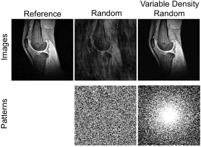
Figure 1.6 Knee Images reconstructed using random and variable density random at an acceleration factor of 2. Use of a variable density random sampling pattern significantly reduces the artifact introduced by undersampling. ... 16

(14)

xiii

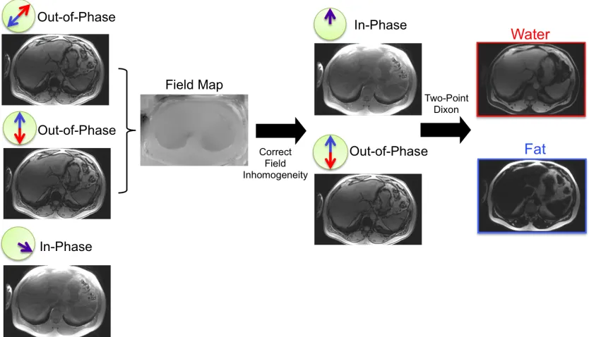
Figure 1.8 Illustration of the Two Point Dixon Method. Water-only and fat-only images are produced by the sum or difference of in-phase and out-of-phase images. ... 19

Figure 1.9 Illustration of the three-point Dixon technique. At each voxel, the difference in phase between the two out-of-phase images is only due to B0 inhomogeneity. By using two

out-of-phase images an estimate the field map, a measure of the B0 inhomogeneity, can be

made. This field map is used to correct the phases of the in-phase and out-of-phase images. The two-point Dixon technique is now used on the corrected images. ... 20

Figure 1.10 IDEAL water-fat separation technique. Images are acquired with at least three different echo times (with different phases between fat and water). A process of updating the field map followed by a least squares decomposition to produce water-only and fat-only images is repeated until the convergence has been achieved. ... 21

Figure 1.11a) Simulated fat and water signal behaviour of a SPGR sequence as a function of flip angle assuming T1,fat=382ms, T1,water=809ms, and TR=10ms. b) Simulated fat fraction at

flip angles of 5°,10°, and 20°. As flip angles increases, the deviation between measured fat fraction and actual fat fraction increases. ... 22

Figure 1.12 Spectrum of a peanut oil phantom. This spectrum shows that fat spectra consist of multiple spectral peaks. ... 23

Figure 1.13 Spectrum of a mouse liver after injection of [1-13C] pyruvate. The peaks at 12.7ppm, 8.6ppm, 5.9ppm, 0ppm correspond to lactate, pyruvate-hydrate, alanine, and

pyruvate. No bicarbonate (~ -10.6ppm) is observed in this spectrum. ... 26

Figure 1.14 Metabolic pathways of [1-13C] Pyruvate. Under anaerobic conditions elevated lactate levels are caused by the conversion of [1-13C] pyruvate into [1-13C] lactate by the enzyme lactate dehydrogenase. Under aerobic conditions, pyruvate and Coenzyme A (CoA) are converted into Acetyl CoA and 13CO2 by pyruvate dehydrogenase. The 13CO2 can

then form 13C-bicarbonate through carbonic anhydrase. [1-13C] pyruvate can be converted into the amino acid [1-13C] alanine through alanine transaminase. ... 27

(15)

xiv

Figure 2.3 SNR maps with net acceleration factor of 2.9 showing the trade-off between spatial resolution and noise as the number of replicas and the volume used to calculate the noise [ni,nj,nk] are changed. The single replica with box size of [0,0,0] is left blank because a

SNR map cannot be calculated under those conditions. ... 44

Figure 3.1 Sample TR of the fat-water pulse sequence. Small y and z gradients are applied during the frequency rewinder, allowing each echo to have a different k-space sampling pattern, thereby improving temporal incoherence. These small gradients are not shown to scale. ... 57

Figure 3.2 Water, Fat and R2* images of 3D abdominal data using the proposed method with

and without R2* correction on data retrospectively undersampled at an acceleration factor

(AF) of 3.2. Reference images (AF=1) were obtained using a fully sampled R2* corrected

IDEAL reconstruction. Arrows point to the spine, a region with high R2* values, which result

in inaccurate fat-water measurements when left uncorrected. ... 61

Figure 3.3 Fat fraction images of 3D abdominal data using the proposed method (bottom row) and sequential parallel imaging and water-fat separation (top row) at acceleration factors (AF) of 1, 4.2, and 5.0. Poisson disk (different pattern for each echo) and uniform (same pattern for each echo) undersampling patterns were used for the proposed method and parallel imaging respectively. ... 62

(16)

xv

factor was fixed for both acquisitions at 4.0. A low contrast object with improved visibility is circled. ... 63

Figure 3.5 A comparison of retrospectively and prospectively decimated water and fat images. The fully sampled dataset was retrospectively decimated using the same sampling pattern (Poisson Disk, net acceleration factor = 3.8) as the prospectively decimated datasets. The equivalence of the two datasets shows that the additional y and z gradients are not

affecting the quality of the water-fat separation. ... 64

Figure 3.6 A prospectively undersampled dataset of entire abdominal cavity reconstructed with the proposed method. A sagittal reformat of the fat images is shown (a). Fat and water images are shown for slices 30, 60, and 90 (b). These three slices correspond to the three horizontal lines in (a). Net acceleration factor for this acquisition was 7.0. ... 65

Figure 3.7 Water and fat images of 32 coil, 3D abdominal data with (8 virtual coils) and without (32 coils) coil compression. Water and fat difference images (amplified by a factor of 10) show the accuracy of the coil compression. Images were acquired at a net acceleration factor of 3.1. ... 66

Figure 4.1 Digital phantom simulation of metabolite separation. Metabolite images with chemical shifts corresponding to pyruvate, pyruvate hydrate, lactate, alanine, and bicarbonate were reconstructed using the proposed reconstruction for cases of low and high B0

inhomogeneity. For each case, metabolite images were reconstructed assuming a constant field map and a spatially varying field map. ... 83

Figure 4.2 Four 13C enriched phantoms containing alanine, lactate, formic acid, and lactate separated using the proposed reconstruction. Results show uniform separation of each component. Formic acid consists of two equal spectral components (doublet). As expected the proposed reconstruction broke the two components of formic acid into two equal

components. ... 84

(17)

xvi

images of a 3D mouse dataset prospectively undersampled at an acceleration factor of 2. .... 87

Figure 4.6 Dynamic metabolite maps acquired using high performance insert gradients at 15s, 25s, and 35s after start of injection. Pyruvate was normalized by a factor 4, alanine, lactate, and bicarbonate images are shown over two coronal slices, one through the heart and the other through the kidneys. The two slices were scaled differently for improved dynamic range in the display of the metabolic signals. In addition, the first pyruvate image acquired at 15s after injection was scaled down by an additional factor of 2 (total 8) for improved

dynamic range. ... 88

Figure 4.7 Metabolite map of the heart at the 25s time point from the dynamic dataset acquired using high performance insert gradients shown in Figure 4.6. The reconstructed metabolite maps using a constant and spatially varying field map show significantly

(18)

xvii

Glossary

3D Three dimensional

2D Two dimensional

AF Acceleration Factor

BW Acquisition bandwidth

CS Compressed Sensing

DESPOT Driven equilibrium single pulse observation of T1/T2

ΔTE Echo spacing

ETL Echo train length

FOV Field of view

γ Gyromagnetic ratio

GRAPPA Generalized autocalibrating partially parallel acquisitions

Hz Hertz

IDEAL Iterative Decomposition of water and fat with Echo Asymmetric and Least-squares estimation

MRI Magnetic resonance imaging

ORF Outer Reduction Factor

PMRI Parallel magnetic resonance imaging

R2* Effective transverse relaxation time

ROI Region of interest

(19)

xviii

TR Repetition time

(20)

Chapter 1

1 Introduction

Magnetic resonance imaging (MRI) is a non-invasive imaging modality based on the interaction of nuclear spins, typically from the 1H of water and fat, with an external magnetic field. MRI is routinely used in clinical practice and offers several advantages over other imaging modalities including no ionizing radiation and excellent soft tissue contrast. The signal (and phase of signal) of magnetic resonance (MR) images is sensitive to many different physiologic and user defined parameters. This sensitivity can be exploited allowing different types of contrast to be generated.

One form of MRI is chemical shift imaging. In this technique, the different resonance frequencies of chemical species (known as a chemical shift) are exploited to separate the signal from each chemical species. This separation is achieved by encoding the MR images in additional dimension, a spectral dimension called the chemical shift dimension. This chemical shift dimension is sampled by acquiring images at different echo times. The sampling of this additional dimension is time-consuming and can limit the resolution and spatial coverage achievable.

The predominant use of chemical shift imaging is water-fat imaging. In this technique, the signal from water is separated from the signal from fat resulting two images: a water-only image and a fat-water-only image. Clinically, water-fat imaging is used in imaging of organs such as the liver, heart, and spine for applications such quantitative grading and staging of non-alcoholic fatty liver disease (1), quantification of fat in bone marrow (2,3), measurement of total visceral adipose tissue (4), detection of brown fat (5,6), and detection of myocardial fat infiltration (7).

(21)

conventional approaches thereby accelerating image acquisition times.

In this chapter, I introduce MR spatial encoding, existing image acceleration techniques, water-fat imaging, and hyperpolarized 13C imaging.

1.1 Spatial Encoding

Three types of magnetic fields are used in MRI to produce an image: the main magnetic field, radiofrequency pulses, and gradients. The main magnetic field polarizes the magnetic moments of 1H leading to a net magnetization aligned along the direction of the

magnetic field, the radiofrequency-pulse tilts this net magnetization into the transverse

plane allowing a nearby coil to detect a signal, and the gradients allow us to resolve

spatially where the measuredsignal is coming from. In this section, the process of spatial

localization by means of gradients is described.

In the presence of a main magnetic field and absence of gradients, all 1_{H will precess}

about the main magnetic field (B0) at the Larmor frequency (ω0):

𝜔! =𝛾𝐵! 1.1

where γ is the gyromagnetic ratio. After demodulation of ω0, the detected signal by a

(22)

𝑆∝ 𝜌(𝑥,𝑦)𝑑𝑥𝑑𝑦. 1.2

Under these conditions, the spatial location of the signal cannot be determined.

1.1.1 Frequency Encoding

The spatial location of the spin densities can be resolved in one dimension (x dimension) through a process called frequency encoding. In this process an additional linearly varying magnetic field called a gradient is superimposed onto main magnetic field. In the presence of this gradient (Gx), the precessional frequency will now vary as a function of

position (x):

𝜔(𝑥)= 𝛾(𝐵!+𝐺!(𝑡)𝑥). 1.3

At any time t, the distribution of frequencies caused by the gradient will result in additional accrual of phase (Δφf)

∆𝜙! 𝑥,𝑡 = −𝑥𝛾 _!!𝐺! 𝑡! 𝑑𝑡′. 1.4

After demodulation of ω0, the detected signal is now the integral of the product of the

spin density and this gradient induced phase term:

𝑆∝ 𝜌(𝑥,𝑦)𝑒!𝒊∆𝝓𝒇(𝒙,𝒕)𝑑𝑥𝑑𝑦 _1.5

Alternatively, Eqn. 1.5can be described in terms of spatial frequency

𝑆(𝑘_!)∝ 𝜌(𝑥,𝑦)𝑒!!!!(!!!)𝑑𝑥𝑑𝑦 1.6

where kx the spatial frequency in the x-direction:

𝑘_! = 𝛾

2𝜋 𝐺(𝑡!)𝑑𝑡′

!

(23)

1.1.2 Phase Encoding

The spatial location of the spin density can be obtained in the y dimension using phase encoding. In this process a gradient is briefly applied in the y direction in-between excitation and the acquisition of signal. Again, the presence of this gradient (Gy) causes

the precessional frequency to vary as a function of position (y):

𝜔(𝑦) =𝛾(𝐵!+𝐺!(𝑡)𝑦). 1.9

Applying a phase encoding gradient for a duration Δt prior to an acquisition results in the

spin density accumulating spatially varying phase (Δφp):

∆𝜙_! 𝑦 =−𝑦𝛾 ∆!𝐺_! 𝑡!

!

𝑑𝑡′ 1.10

This phase accrual is identical to that seen in Eqn 1.4. After demodulation of ω0, the

detected signal is now the integral of the product of the spin density and frequency and phase gradient induced phase terms:

𝑆∝ 𝜌(𝑥,𝑦)𝑒!𝒊(∆𝝓𝒇 𝒙,𝒕!∆𝝓𝒑 𝒚,𝒕)_{𝑑𝑥𝑑𝑦} _1.11

or

𝑆(𝑘!,𝑘!)∝ 𝜌(𝑥,𝑦)𝑒!!!!(!!!!!!!)𝑑𝑥𝑑𝑦 1.12

(24)

_𝑘_! ₌ !

!! 𝐺!(𝑡

!_)𝑑𝑡′

!

! . 1.13

By means of a two-dimensional inverse Fourier transform, the spin density can be resolved in the x dimension:

_𝜌 _𝑥,_𝑦 _∝ _𝑆 _𝑘

!,𝑘! 𝑒!!!(!!!!!!!)𝑑𝑘!𝑑𝑘!. 1.14

Equation 1.14 states that if measurements of the signal are made at different spatial frequency kx and ky, then spin density can be resolved in the x and y direction. In order

to acquire different ky spatial frequency, repeated frequency encoded acquisitions using

different Gy gradients (Eqn. 1.13) are required. This repetitive process limits the speed

MR images can be acquired.

1.1.3 k-space

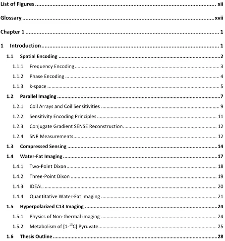
Figure 1.1 summarizes the encoding process. In the absence of gradients (Figure 1.1), only the center point of k-space is sampled. This results in signal that cannot be spatially resolved. By applying a frequency gradient and acquiring data throughout the duration of the gradient (Figure 1.1b), the center line of k-space is now sampled resulting in signal that can be resolved in one dimension. Resolving an image in two dimensions requires the use of phase encoding gradients. The application of a phase encoding gradient in the y direction prior to applying frequency encoding results in a off-centered line of k-space being sampled. Repeated acquisitions in the presence of different phase encoding gradients will sample ky space. Once the ky dimension has been adequately sampled, the

(25)

Figure 1.1 The encoding process. a) In the absence of gradients, only the central point of k-space can be sampled. As a result signal cannot be spatially resolved. b) Application of a frequency encoding gradient allows the central line of k-space to

be sampled and the image to be resolved in the frequency encode direction. c) To resolve the entire image, the entire k-space must be sampled. Repeated acquisitions

(26)

1.2 Parall

el Imaging

Magnetic Resonance (MR) images are acquired by sampling a Fourier space known as k-space where the spacing between adjacent samples in k-k-space (Δk) defines the field of view (FOV) of the image

𝐹𝑂𝑉 = 1

∆𝑘 1.15

and the largest k-space position measured (kx,max, ky,max) defines its resolution

𝛿 = 1

2𝑘_!"# 1.16

Figure 1.2 illustrates these principles. For a given field of view and resolution, the

number of phase encodes required is fixed. In parallel imaging, a portion of the k-space phase encodes is not sampled which should result in an aliased image (Figure 1.2b).

(27)

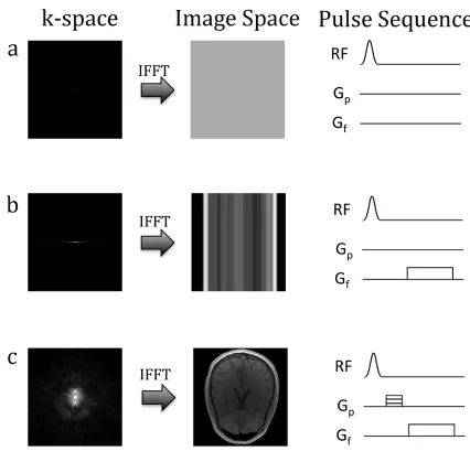
Figure 1.2 Relationship between k-space and image space. a) The field-of-view of an

image is proportional to the inverse of the spacing between adjacent samples (Δk)

while the resolution is proportional to the max k-space position. b) In the case where only half of the phase encodes are acquired, the final image will be a

field-of-view reduced by a factor of two resulting in aliasing.

Parallel imaging techniques fall into one of two categories: k-space (8,9) and

image-space techniques (10). In k-space techniques, the missing k-space lines are reconstructed

and an inverse Fourier transform results in the reconstructed image. In image-space

techniques, the undersampled k-space is Fourier transformed to give an aliased image.

The aliased image is then un-aliased by means of the coil sensitivity to reconstruct the

(28)

parallel imaging reconstruction, and methods to measure SNR in parallel imaging will be described.

1.2.1 Coil Arrays and Coil Sensitivities

Arrays of surface coils can offer significant advantages in MR acquisitions including higher SNR and accelerated image acquisition through the use of parallel imaging. Each surface coil has a non-uniform receive profile, known as its coil sensitivity, which modulates the signal intensity across the field of view. Therefore, the signal intensity S(r) measured at any position r will be the product of the coil sensitivity C(r) and the underlying spin density ρ(r):

𝑆 𝒓 ∝𝐶(𝒓)𝜌(𝒓) 1.17

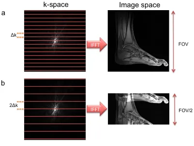
Figure 1.3 shows the coil sensitivities and resulting coil and coil-combined images for an 8 channel torso array.

(29)

Figure 1.3 Four coil sensitivities, individual coil images, and the coil-combined image for an 8 channel torso array. Signal variation across the field of view caused

by the coil sensitivity results in elevated signal intensity in locations near each surface coil and low signal intensities in locations far from each surface coil.

(30)

In the root sum square approach, the root-sum square (RSS) of the each of the surface coils is calculated resulting in an image that is roughly uniform. The coil sensitivity is then estimated as the ratio of the signal intensity of the surface coil and the RSS image. For a small number of coils (ie. <8 coils), the assumption that the RSS image has uniform signal intensity (ie. no coil sensitivity weighting) is a good approximation. However, for large arrays this assumption breaks down in regions near the coils, resulting in errors in the coil sensitivity estimations.

1.2.2 Sensitivity Encoding Principles

In the case that surface coils are used, Eqn. 1.14 needs to be modified to account for the coil sensitivity. The signal measured at k-space position k by the lth receive coil can be described as

𝑆_! 𝒌 = 𝜌(𝒓)𝐶_!(𝒓)𝑒!𝒊𝟐𝝅(𝒌∙𝒓)_𝑑_𝒓 _1.18

where ρ(r) is the spin density and Cl(r) is the coil sensitivity. Combining the coil

sensitivity and Fourier encoding creates encoding functions that differ for each coil:

𝐸_! 𝒌,𝒓 ≡ 𝐶_!(𝒓)𝑒!!!!(𝒌∙𝒓) _1.19

Alternatively, Eqn. 1.18 can be discretized and described in matrix form:

_𝑆

! = 𝐸!"𝜌! !

_1.20

𝑺=𝐸𝝆 1.21

where S is a vector of k-space values with element Sq=Sl(k) such that every combination

of k-space index, k, and coil index, l, map onto index q, ρ is a vector of spin density with elements ρp at position index p, and E is the encoding matrix, consisting of the coil

sensitivity and Fourier encoding, a matrix with elements

(31)

achieved after relatively few iterations, significantly reducing reconstruction times (13).

1.2.4 SNR Measurements

The cost of acceleration using parallel imaging is reduced SNR resulting from two effects: reduced signal averaging results in a loss of SNR by a factor of the square root of the acceleration factor and an additional penalty called the g-factor (10) which describes the additional noise amplification caused by the parallel imaging reconstruction. This g-factor is dependent on the sampling strategy and the design of the coil array (number of coils and geometry of the coils in the array). In addition, this g-factor penalty varies spatially making the conventional method for SNR measurement, which relies on a ROI from a signal free region to estimate the noise, invalid. Existing methods for measuring SNR in a parallel imaging reconstruction include direct SNR calculations (7,10), multiple pseudo-replica (14), and estimation from multiple acquisitions (15-17).

Analytical methods for “direct SNR calculation” have been proposed (7,10). Here, direct inversion of the encoding matrix allows SNR scaled images to be reconstructed. However, inversion of the encoding matrix is not computationally feasible for an arbitrary sampling pattern or parallel imaging reconstruction. Typically this method has been restricted to uniform or 1d undersampling patterns, situations where this inversion can be simplified.

(32)

replica images is taken to produce a difference image. Image noise can then be estimated from ROIs within the difference images using the following formula

𝑁𝑜𝑖𝑠𝑒= (𝑉(𝑖,𝑗+1)−𝑉(𝑖,𝑗))

!

!!!

!

!!!

4 ! (𝑚−1)

!!!

1.23

where n and m are the number of rows and columns within the ROI and V(i,j) is the signal intensity of the difference image at pixel location [i,j]. These techniques assume that each replica is identical except for the noise, making these techniques sensitive to variations between acquisitions (such as motion and radiofrequency instability). In particular, sensitivity to motion (even motion on the order of a voxel) makes repeated acquisition techniques impractical for in vivo imaging.

(33)

Figure 1.4 Flowchart of the multiple-pseudo replica method.

1.3 Compressed Sensing

(34)

Figure 1.5 Sparsity of a liver dataset in the wavelet domain. Images reconstructed using the largest 15% of the wavelet coefficients and 100% of the coefficients show

excellent agreement.

The first requirement for a CS reconstruction is that the MR image must be sparse in a known transform domain. Sparsity refers to the ability of an image to be described by relatively few non-zero coefficients. Typically transform sparsity rather than image sparsity is enforced, meaning that the image can be described by a few non-zero coefficients in a transform domain. Two commonly used transform domains for MR images are wavelet and finite difference. In Figure 1.5, the sparsity of a liver dataset in the wavelet domain is shown. Using the largest 15% of the coefficient in the wavelet domain, the image can be recovered with excellent fidelity.

(35)

Figure 1.6 Knee Images reconstructed using random and variable density random at an acceleration factor of 2. Use of a variable density random sampling pattern

significantly reduces the artifact introduced by undersampling.

The final requirement is a non-linear reconstruction that enforces both sparsity of the reconstructed image and consistency of the reconstructed image with the acquired data. This criterion can be meet by solving the following convex optimization problem:

𝑎𝑟𝑔𝑚𝑖𝑛

𝑚 = ||𝐹!𝑚−𝑦||!!+𝜆||Ψ𝑚||! 1.24

where FU is the undersampled Fourier operator, m is the image, y is the undersampled

(36)

Compressed sensing has been shown to be a complimentary approach to parallel imaging for image acceleration (20,21). In such methods, Fourier encoding is again replaced with the hybrid encoding described by Eqn. 1.19 in a non-linear reconstruction that promotes sparsity. The combination of both parallel imaging and compressed sensing has been shown to reduce the g-factor penalty paid by parallel imaging reconstructions. Using both, acceleration factors can be achieved that are higher than either compressed sensing or parallel imaging on their own.

1.4 Water

-

Fat Imaging

Water and fat are the two prominent sources of signal in in vivo applications of MRI. Water and fat exhibit a difference in resonance frequencies called a chemical shift. Electrons surrounding any molecule shield the hydrogen nuclei from an external magnetic field causing small but measurable perturbations in the magnetic field experienced by the 1H nuclei. These perturbations to the magnetic field are different for fat and water molecules and result in resonance frequencies that differ by 3.4ppm (22,23). At 3T, this results in a 434Hz difference between the resonance frequency of water and fat (Figure 1.7). This difference can be exploited, allowing separation of signal due to water from signal due to fat.

(37)

Figure 1.7 Spectrum taken from the liver of a patient with non-alcoholic fatty liver disease. The spectrum shows the 3.4ppm chemical shift between water (left) and fat

(right).

1.4.1 Two-Point Dixon

At any particular pixel p and echo time t, the total signal Sp(t) can be considered as the

sum of the signal from fat protons, ρ_f,p_{, with the signal from water protons,}ρ_w,p_:

𝑆_!(𝑡)= 𝜌_!_,_!+𝜌_!_,_!𝑒!!!"#$ _1.25

where Δf is the chemical shift between water and fat. At t=0, the transverse components of fat and water are in phase with one another (24). As time progresses, the fat and water signal will dephase due their chemical shift. If two images are acquired at echo times

when the water and fat signal are in-phase (SIP) and 180◦ out-of-phase (SOP), then simple

addition and subtraction of the in-phase and out-of-phase images results in a water-only and fat-only images (25):

𝑆_! = 1

2(𝑆!"+𝑆!") 1.26

𝑆! =

1

(38)

Figure 1.8 Illustration of the Two Point Dixon Method. Water-only and fat-only images are produced by the sum or difference of in-phase and out-of-phase images.

Figure 1.8 demonstrates this technique using in-phase and out-of-phase images taken from the abdomen. This approach assumes that the magnetic field is homogeneous, an assumption that in practice is never true.

1.4.2 Three-Point Dixon

In the presence of non-uniform magnetic field, additional phase will accumulate due to the magnetic field inhomogeneity:

𝑆!(𝑡)= (𝜌!,!+𝜌!,!𝑒!!!"#$)𝑒!!!!!! 1.28

Here ψp is the field map, a measure of B0 inhomogeneity in units of Hz. Under such

(39)

Figure 1.9 Illustration of the three-point Dixon technique. At each voxel, the difference in phase between the two out-of-phase images is only due to B0 inhomogeneity. By using two out-of-phase images an estimate the field map, a measure of the B0 inhomogeneity, can be made. This field map is used to correct the

phases of the in-phase and out-of-phase images. The two-point Dixon technique is now used on the corrected images.

1.4.3 IDEAL

(40)

Figure 1.10 IDEAL water-fat separation technique. Images are acquired with at least three different echo times (with different phases between fat and water). A process of updating the field map followed by a least squares decomposition to produce water-only and fat-only images is repeated until the convergence has been

achieved.

1.4.4 Quantitative Water-Fat Imaging

The clinical need for techniques to quantify fat has driven the development of quantitative chemical shift based water-fat techniques. The proton density fat-fraction (PDFF) defined as the ratio of the density of mobile protons from fat to the total density of mobile protons from both fat and water has emerged as the most commonly used and most biologically relevant imaging biomarker for tissue fat concentration (30). Unfortunately, many factors affect the signal intensities of fat and water. These confounding factors result in biased estimates of the PDFF and must be accounted for in order to achieve accurate estimates. These factors include T1 bias (31,32), accurate

(41)

Figure 1.11a) Simulated fat and water signal behaviour of a SPGR sequence as a function of flip angle assuming T1,fat=382ms, T1,water=809ms, and TR=10ms. b)

Simulated fat fraction at flip angles of 5°,10°, and 20°. As flip angles increases, the

deviation between measured fat fraction and actual fat fraction increases.

T1 bias in the PDFF arises from the difference in T1 of fat and water. In Figure 1.11a

shows the behaviour of fat and water signals as a function of flip angles assuming T1,fat=382ms and T1,water=809ms for a spoiled gradient echo sequence (SPGR). At higher

flip angles the water and fat signals becomes more T1 weighted (Figure 1.11a), resulting

in an increased bias in the fat fraction measurement (Figure 1.11b). Therefore, a small flip angle is used to minimize T1 effects, resulting in reduced bias in the PDFF at the cost

of reduced SNR. Alternative approaches have been proposed that use multiple acquisitions at different flip angles to measure the T1 of fat and water (31,35). However,

(42)

Figure 1.12 Spectrum of a peanut oil phantom. This spectrum shows that fat spectra consist of multiple spectral peaks.

The previously defined signal model Eqn. 1.28 assumes the water and fat spectra are singlets. While this is a good assumption for water, Figure 1.12 shows that the spectrum of fat is complex, consisting of multiple spectral peaks. These additional spectral peaks lead to bias in our fat and water estimates. A more accurate spectral model should contain the additional spectral peaks of fat:

_𝑆

!(𝑡) =(𝜌!,!+𝜌!,! 𝛼!𝑒!!!"!!! !

)𝑒!!!!𝒑!

1.29

where αj and fj are the relative amplitudes and chemical shifts, respectively, of the jth spectral peak of fat. The amplitude of each spectral peak of fat could be estimated using IDEAL provided that enough echo images were acquired. Typically, the relative amplitude and frequency of each spectral component of fat is assumed to be known a priori.

Unlike the previous discussed confounding factors, T2* effects cannot be accounted for

using appropriate imaging parameters or prior knowledge. An additional free parameter must be added to the signal model to account for the R2* decay (23,33):

𝑆!(𝑡) =(𝜌!,!+𝜌!,! 𝛼!𝑒!!!"!!! !

)𝑒!!!(!!!!!,!

∗

(43)

state can be produced (37). This hyperpolarized state offers signal enhancement on the order of 10,000 fold over thermal imaging and enhances imaging of 13C substrates (37). The polarized substrates are injected and their metabolic by-products detected. The following sections will discuss: the physics of non-thermal imaging and its impact on

imaging strategies and the biochemistry of the most commonly used substrate [1-13C] pyruvate.

1.5.1 Physics of Non-thermal imaging

Many nuclei (eg. 1_H,3_He,13_C,129_{Xe) have a non-zero spin that can be detected by NMR}

and MRI through the interaction of a nuclear spin with an external magnetic field. For nuclei with a spin quantum number of ½ (e.g. 1H, 13C), the interactions of spins with an external magnetic field results in two possible spin states, namely, parallel alignment and anti-parallel alignment. The slight preference for any given nuclei to populate the parallel state results in a population difference or polarization P given by:

𝑃= 𝑁!−𝑁!

𝑁!₊_𝑁! ≈

ℎ𝛾𝐵_!

4𝜋𝑘𝑇 1.31

where N+ and N- are the number of spins in the parallel and anti-parallel state, γ is the gyromagnetic ratio of the nuclei, h is Planck’s constant , k is Boltzmann constant, and T is the temperature. This polarization gives rise to detectable signal.

(44)

in vivo nuclei is large due to the high concentration of hydrogen (~88M) (38) and the high natural abundance of the isotope 1H. This makes detection of 1H signal relatively easy despite this low polarization. In 13C MRI the number of spins is much smaller due the lower biological abundance of carbon (approximately 18% by mass) and the low natural abundance of the isotope 13C (1%). As such, detection of 13C signal difficult.

An approach to enhance signal is to temporarily increase the polarization relative to thermal equilibrium resulting in a non-thermal, hyperpolarized state. Polarization increases of more than four orders of magnitude can be obtained through a process called dynamic nuclear polarization (37). In this approach, a 13_{C labeled substrate is polarized}

and subsequently injected into the subject.

The increased polarization due to this hyperpolarized state immediately begins to decay back to thermal equilibrium. The rate of this decay is substrate-dependent and is described by the substrate’s T1. This rapid decay limits the time window in which

hyperpolarized signal can be detected and makes efficient rapid imaging strategies necessary.

1.5.2 Metabolism of [1-

13

C] Pyruvate

[1-13C] pyruvate (pyruvate labeled with 13C in the C1 position) is the most commonly used hyperpolarized substrate for multiple reasons. Its central role in metabolism allows for the detection of metabolites from several different metabolic pathways. In addition, its desirable hyperpolarization properties, such as high polarization levels and a relatively long T1 of ~30s in vivo and ~45s ex-vivo, improve the quality and life-time of

polarization (39,40).

(45)

(46)

Figure 1.14 Metabolic pathways of [1-13C] Pyruvate. Under anaerobic conditions

elevated lactate levels are caused by the conversion of [1-13C] pyruvate into

[1-13_{C] lactate by the enzyme lactate dehydrogenase. Under aerobic conditions,}

pyruvate and Coenzyme A (CoA) are converted into Acetyl CoA and 13CO2 by

pyruvate dehydrogenase. The 13CO2 can then form 13C-bicarbonate through

carbonic anhydrase. [1-13C] pyruvate can be converted into the amino acid [1-13C]

(47)

In Chapter 3, an integrated compressed sensing, parallel imaging, R2* corrected water-fat

separation technique for water-fat imaging of highly accelerated acquisitions is described. The technique is demonstrated using a customized IDEAL-SPGR pulse sequence to acquire retrospectively and prospectively undersampled datasets of the liver, calf, knee, and abdominal cavity. At high acceleration factors, this technique is shown to offer improved image quality over parallel imaging.

In Chapter 4, an integrated compressed sensing, metabolite separation technique for separation of pyruvate and its metabolites, lactate, alanine, and bicarbonate is described. The technique was validated using phantom and in vivo experiments using a broadbanded variant of the IDEAL-SPGR sequence.

(48)

1.7 References

1. Hussain HK, Chenevert TL, Londy FJ, Gulani V, Swanson SD, McKenna BJ, Appelman HD, Adusumilli S, Greenson JK, Conjeevaram HS. Hepatic fat fraction: MR imaging for quantitative measurement and display--early experience. Radiology 2005;237(3):1048-1055.

2. Schick F, Einsele H, Lutz O, Claussen CD. Lipid selective MR imaging and localized 1H spectroscopy of bone marrow during therapy of leukemia. Anticancer Res 1996;16(3B):1545-1551.

3. Schick F, Weiss B, Einsele H. Magnetic resonance imaging reveals a markedly inhomogeneous distribution of marrow cellularity in a patient with

myelodysplasia. Ann Hematol 1995;71(3):143-146.

4. Kuk JL, Katzmarzyk PT, Nichaman MZ, Church TS, Blair SN, Ross R. Visceral fat is an independent predictor of all-cause mortality in men. Obesity (Silver Spring) 2006;14(2):336-341.

5. Hu HH, Perkins TG, Chia JM, Gilsanz V. Characterization of human brown adipose tissue by chemical-shift water-fat MRI. AJR Am J Roentgenol 2013;200(1):177-183.

6. Hu HH, Yin L, Aggabao PC, Perkins TG, Chia JM, Gilsanz V. Comparison of brown and white adipose tissues in infants and children with chemical-shift-encoded water-fat MRI. J Magn Reson Imaging 2013.

7. Kellman P, McVeigh ER. Image reconstruction in SNR units: a general method for SNR measurement. Magn Reson Med 2005;54(6):1439-1447.

(49)

2010;207(1):59-68.

12. McKenzie CA, Yeh EN, Ohliger MA, Price MD, Sodickson DK. Self-calibrating parallel imaging with automatic coil sensitivity extraction. Magn Reson Med 2002;47(3):529-538.

13. Pruessmann KP, Weiger M, Bornert P, Boesiger P. Advances in sensitivity encoding with arbitrary k-space trajectories. Magn Reson Med 2001;46(4):638-651.

14. Robson PM, Grant AK, Madhuranthakam AJ, Lattanzi R, Sodickson DK,

McKenzie CA. Comprehensive quantification of signal-to-noise ratio and g-factor for image-based and k-space-based parallel imaging reconstructions. Magn Reson Med 2008;60(4):895-907.

15. NEMA. Determination of signal-to-noise ratio (SNR) in diagnostic magnetic resonance imaging. Rosslyn, VA; 2001.

16. Reeder SB, Wintersperger BJ, Dietrich O, Lanz T, Greiser A, Reiser MF, Glazer GM, Schoenberg SO. Practical approaches to the evaluation of signal-to-noise ratio performance with parallel imaging: application with cardiac imaging and a 32-channel cardiac coil. Magn Reson Med 2005;54(3):748-754.

(50)

18. Taubman D, Marcellin M. Image compression fundamentals, standards and practice. Kluwer Internation Series in Engineering and Computer Science: Kluwer Academic Publishers; 2002.

19. Lustig M, Donoho D, Pauly JM. Sparse MRI: The application of compressed sensing for rapid MR imaging. Magn Reson Med 2007;58(6):1182-1195.

20. Lustig M, Alley M, Vasanawala S, Donoho D, Pauly JM. L1 SPIR-iT:

Autocalibrating Parallel Imaging Compressed Sensing. Proceedings of the 17th Annual Meeting of ISMRM, Honolulu, USA 2009:379.

21. Liang D, Liu B, Wang J, Ying L. Accelerating SENSE using compressed sensing. Magn Reson Med 2009;62(6):1574-1584.

22. Hamilton G, Yokoo T, Bydder M, Cruite I, Schroeder ME, Sirlin CB, Middleton MS. In vivo characterization of the liver fat (1)H MR spectrum. NMR Biomed 2011;24(7):784-790.

23. Yu H, Shimakawa A, McKenzie CA, Brodsky E, Brittain JH, Reeder SB. Multiecho water-fat separation and simultaneous R2* estimation with

multifrequency fat spectrum modeling. Magn Reson Med 2008;60(5):1122-1134.

24. Bydder M, Yokoo T, Yu H, Carl M, Reeder SB, Sirlin CB. Constraining the initial phase in water-fat separation. Magn Reson Imaging 2011;29(2):216-221.

25. Dixon WT. Simple proton spectroscopic imaging. Radiology 1984;153(1):189-194.

26. Glover GH, Schneider E. Three-point Dixon technique for true water/fat decomposition with B0 inhomogeneity correction. Magn Reson Med 1991;18(2):371-383.

(51)

2012;36(5):1011-1014.

31. Liu CY, McKenzie CA, Yu H, Brittain JH, Reeder SB. Fat quantification with IDEAL gradient echo imaging: correction of bias from T(1) and noise. Magn Reson Med 2007;58(2):354-364.

32. Bydder M, Yokoo T, Hamilton G, Middleton MS, Chavez AD, Schwimmer JB, Lavine JE, Sirlin CB. Relaxation effects in the quantification of fat using gradient echo imaging. Magn Reson Imaging 2008;26(3):347-359.

33. Yu H, McKenzie CA, Shimakawa A, Vu AT, Brau AC, Beatty PJ, Pineda AR, Brittain JH, Reeder SB. Multiecho reconstruction for simultaneous water-fat decomposition and T2* estimation. J Magn Reson Imaging 2007;26(4):1153-1161.

34. Chebrolu VV, Hines CD, Yu H, Pineda AR, Shimakawa A, McKenzie CA, Samsonov A, Brittain JH, Reeder SB. Independent estimation of T*2 for water and fat for improved accuracy of fat quantification. Magn Reson Med

2010;63(4):849-857.

35. Karampinos DC, Yu H, Shimakawa A, Link TM, Majumdar S. T(1)-corrected fat quantification using chemical shift-based water/fat separation: application to skeletal muscle. Magn Reson Med 2011;66(5):1312-1326.

(52)

Spoiled Gradient Imaging. Proceedings of the 17th Annual Meeting of ISMRM, Honolulu, USA 2009:656.

37. Ardenkjaer-Larsen JH, Fridlund B, Gram A, Hansson G, Hansson L, Lerche MH, Servin R, Thaning M, Golman K. Increase in signal-to-noise ratio of > 10,000 times in liquid-state NMR. Proc Natl Acad Sci U S A 2003;100(18):10158-10163.

38. Haacke EM, Brown RW, Thompson MR, Venkatesan R. Magnetic Resonance Imaging: Physical Principles and Sequence Design. New York: Wiley-Liss; 1999.

39. Ardenkjaer-Larsen JH, Macholl S, Johannesson H. Dynamic nuclear polarization with trityls at 1.2 K. Applied Magnetic Resonance 2008;34(3-4):509-522.

40. Golman K, in 't Zandt R, Thaning M. Real-time metabolic imaging. Proc Natl Acad Sci U S A 2006;103(30):11270-11275.

41. Lee P, Leong W, Tan T, Lim M, Han W, Radda GK. In vivo hyperpolarized carbon-13 magnetic resonance spectroscopy reveals increased pyruvate carboxylase flux in an insulin-resistant mouse model. Hepatology 2013;57(2):515-524.

42. Schroeder MA, Cochlin LE, Heather LC, Clarke K, Radda GK, Tyler DJ. In vivo assessment of pyruvate dehydrogenase flux in the heart using hyperpolarized carbon-13 magnetic resonance. Proc Natl Acad Sci U S A 2008;105(33):12051-12056.

43. Wiesinger F, Weidl E, Menzel MI, Janich MA, Khegai O, Glaser SJ, Haase A, Schwaiger M, Schulte RF. IDEAL spiral CSI for dynamic metabolic MR imaging of hyperpolarized [1-13C]pyruvate. Magn Reson Med 2012;68(1):8-16.

44. Reeder SB, Brittain JH, Grist TM, Yen YF. Least-squares chemical shift

(53)

spatial dependence of noise properties in the reconstructed image prevents the use of the conventional region of interest (ROI) calculations of SNR (where the noise is measured using an ROI in a region containing no signal).

Parallel imaging reconstructions like SMASH (1), SENSE (2) and GRAPPA (3), which use signals simultaneously acquired from multiple receive coils, rely on the spatial information contained in each coil’s unique sensitivity to partially replace conventional phase encoding. The penalty for replacing a portion of the phase encoding is a loss in SNR from two effects: a decrease in SNR by a factor of the square root of the acceleration factor due to reduced signal averaging and an additional penalty caused by spatially dependent noise amplification (the “g-factor”)(2).

A number of alternative methods of measuring SNR for phased array image reconstructions have been proposed, including direct SNR calculation (4), Monte Carlo based “pseudo multiple replica” SNR estimation (5) and estimation of SNR from multiple acquisitions (6). However, each of these methods has limitations, as we will outline below.

Direct SNR calculation (4) can be computationally rapid (ie. calculation does not take substantially longer than the image reconstruction) but is not applicable to sampling

1_{A version of Chapter 2 has been published: Wiens CN, Kisch SJ, Willig-Onwuachi JD, McKenzie CA.}

(54)

patterns and/or reconstruction techniques in which an analytic g-factor map is not computationally feasible. A common case in which direct SNR calculation is not computationally feasible due to the size of the matrix that needs to be inverted is 2D-accelerated generalized SENSE reconstructions with variable density sampling (7).

The pseudo multiple replica method is more broadly applicable than the direct SNR calculation method but can require lengthy reconstruction times. It can be used with any linear image reconstruction, including SENSE and “complex-GRAPPA” with any arbitrary k-space trajectories pattern. The limitations of the pseudo multiple replica method, however, lie in its lengthy computation time, as it requires multiple reconstructions (typically ~128) of the raw dataset with random pseudo-noise added to ensure a precise estimate of SNR.

SNR estimates from multiple image acquisitions (6,8,9) are computationally rapid, but they require substantial additional image acquisition time and are highly susceptible to errors resulting from variations between acquisitions (e.g. motion, radiofrequency instability, etc.). In one multiple acquisition method proposed in the NEMA standard, an image is acquired twice and the difference between the two images is used to determine the noise (6). Motion, even on a sub-pixel level, will introduce error in the SNR estimate, making this method difficult for in vivo imaging.

(55)

replica method (5) works on the same assumption, but introduces the idea that synthetic noise that has been correctly scaled and correlated between elements can be repeatedly added to a single dataset to produce the same noise statistics on a pixel-by-pixel basis by analyzing a stack of reconstructed pseudo images. Note that because the added noise is correlated and scaled appropriately and has passed through the same signal reconstruction algorithm, each pseudo-image has the same spatial noise amplification as the original image without synthetic noise.

A noise map can be calculated by taking the standard deviation through a stack of replicas (actual or synthetic) for each pixel

,

2.1

where V is the real (or equivalently imaginary) component of pseudo-image m at spatial position (i,j,k), Vave is the average value through the stack of replicas of the real (or

imaginary) component,

,

2.2 Noise(i,j,k)=

(V(i,j,k,m)−V_ave(i,j,k))2

m=1

nreplicas

∑

nreplicas −1

Vave(i,j,k)=

V(i,j,k,m)

m=1

n_replicas

∑

(56)

and nreplicas is the number of replicas. This stack of replicas can be produced using

pseudo-images, actual replicas, or a combination of both. This method requires at least two replicas with the cost of fewer replicas being a decrease in precision.

Traditionally, however, SNR has been measured by examining spatial noise variations (i.e. with fixed ROIs). If we include nearby pixels with a sliding window average method to obtain additional noise statistics, Eqn. 2.1 can be further generalized. Here image noise is calculated using a 4D moving standard deviation calculation:

,

2.3

where we now use nearby pixels of a sliding 3D volume of interest (VOI) with dimensions (2ni+1) x (2nj+1) x (2nk+1) to obtain additional noise statistics. In other

words, for each pixel, noise statistics are determined by examining the set of pixels in the

local VOI for all replicas. Thus for each pixel has been computed as the average of that same set of pixels—not just over the replica dimension.

.

2.4

Problems arise with Eqn. 2.3 when the signal varies across the VOI and results in biased noise calculations. To remove this problem, the noise is calculated on noise-only images rather than the pseudo-images as done in the method describe in the NEMA standard (6). Noise-only images are produced by subtracting the pseudo-images from the original image with no synthetic noise added and will subsequently be denoted N. Equation 2.3 can be now be written in terms of noise-only images

Noise(s,q,r)=

(V(i,j,k,m)−V(s,q,r))2

m=1

nreplicas

∑

k=r−nk

r+nk

∑

j=q−nj

q=nj

∑

i=s−ni

s+ni

∑

n_replicas(2n_i +1)(2n_j +1)(2n_k+1)−1

V

V(s,q,r)=

V(α,β,γ,m)

m=1

n_replicas

∑

γ=r−n_k r+n_k

∑

β=q−n_j q+n_j

∑

α=s−n_i s+n_i

∑

(57)

.

The use of nearby pixels allows the use of fewer replicas without the loss in precision. The sliding volume of interest calculation allows for the noise to vary across the image, but the use of nearby pixels for noise calculation causes some spatial smoothing of the noise map. Large g-factor spikes will be measured multiple times by nearby pixels, effectively blurring the spikes over the volume used to calculate the noise. It is desirable to have a box size that is large enough to provide reasonable statistics for noise calculation but small enough so that there is minimal variation in the g-factor over its volume. The number of replicas and the sliding volume of interest box size can be adjusted in combination to achieve the desired/acceptable level of noise accuracy, spatial smoothing, and computation time.

In the limiting case of only one replica (nreplicas = 1) noise is measured spatially and Eqn.

2.5 simplifies to a moving VOI standard deviation calculation:

.

2.7

The generalized pseudo replica method of calculating an SNR map involves calculating a noise map using Eqn. 2.5 then dividing the magnitude of the original image by this noise map on a pixel-by-pixel basis.

n_replicas(2n_i +1)(2n_j+1)(2n_k+1)

Noise(s,q,r)=

N(i,j,k)−N

(

)

2

k=r−nk r+nk

∑

j=q−nj q+nj

∑

i=s−ni s+ni

∑

(58)

2.3 Methods

2.3.1 Phantom Experiments

The generalized pseudo replica method of SNR estimation was first validated for 1D acceleration on a spherical phantom by comparison with the pseudo-replica and analytic direct SNR methods. A fully gradient encoded 3D spoiled gradient recalled echo (SGPR) dataset was acquired of a spherical phantom using an eight channel head coil at 3T (MR 750, GE Healthcare, Waukesha, WI, USA). The k-space data were decimated to obtain sampling patterns with net acceleration factors of 1.8 (outer reduction factor (ORF) of 2 and 32x32 fully sampled center lines) and 2.9 (outer acceleration factor of 4 and 32x32 fully sampled center lines). Imaging parameters were as follows: TE=1.7 ms, TR=5.0 ms, matrix size=256x256x64, field of view (FOV) 220 mm, slice thickness=3.5 mm, flip angle=15°, and bandwidth (BW)= +/- 143 kHz.

2.3.2 in vivo

Experiments

The generalized pseudo replica method was also compared to the standard pseudo multiple replica method for a two dimensional, variable density undersampling pattern in vivo. After obtaining ethics approval from the University of Western Ontario’s Research Ethics Board and informed consent from a healthy volunteer, one low resolution, fully encoded data set and two high resolution, undersampled 3D SGPR datasets of the liver were acquired using a 32 channel torso coil at 3T (MR 750, GE Healthcare, Waukesha, WI, USA). The fully sampled dataset was taken at a lower resolution than the undersampled datasets because image acquisition in the abdomen must be performed in a single breath-hold (~20s) to avoid breathing-induced motion artefacts.

(59)

of the pseudo-noise (5,11)

2.3.4 Image reconstruction and noise analysis

For the 1D-accelerated phantom data, direct matrix-inverse generalized SENSE was used for image reconstruction. SNR maps were calculated using direct SNR (11), pseudo multiple replica (5) with 128 replicas, and generalized pseudo replica methods (as described above in the Theory section) with a single replica. Normalized difference maps were also calculated to compare results from the latter two techniques to the first. For phantom data, the following formula was used

2.8

where A(i,j) is the SNR map from either the pseudo multiple replica technique or the generalized method and B(i,j) is the SNR map from the direct SNR technique.

These difference maps were also characterized numerically. The mean difference from the direct SNR method was calculated for both the pseudo multiple replica and generalized pseudo replica methods (simply the mean of the difference maps described above). Confidence intervals were also tabulated for both methods. The range indicated by the 99% confidence interval is meant to represent the range in which the central 99% of the pixel values for a given difference map fall. The mean difference and confidence intervals were calculated for each acceleration factor presented.

NormalizedDifference(i,j)= A(i,j)−B(i,j)

(60)

For the 2D-acclerated in vivo data, conjugate gradient generalized SENSE was used for image reconstruction. SNR maps were calculated using the pseudo multiple replica method with 128 replicas and using the generalized method with a single replica. The direct SNR method was not calculated in this case, since direct SNR calculation is not computationally feasible for non-uniform, 2D-accelerated acquisitions. Normalized difference maps, calculated from Eqn. 2.8, were used to compare results from these two techniques.

All image reconstructions, calculations, and analyses were performed using MATLAB (R2009-64bit, The MathWorks, Natick, MA, USA) on Mac Pro workstations (Apple Computer, Cupertino, CA, USA).

2.4 Results

Figure 2.1 shows SNR maps calculated using the direct SNR, pseudo multiple replica, and generalized pseudo replica methods for a slice of a spherical phantom reconstructed using a direct inverse generalized SENSE reconstruction. For each method, SNR maps are shown for a fully sampled dataset, an undersampled dataset with a net acceleration factor of 1.8, and an undersampled dataset with a net acceleration factor of 2.9.

(61)

Figure 2.1 SNR maps using direct SNR calculation, pseudo multiple replica with 128 replicas (PR128), and generalized pseudo replica with a single replica (PR1) for generalized SENSE reconstructions with one dimensional net accelerations of 1, 1.8, and 2.9. Normalized differences between pseudo multiple replica and Direct SNR as well as generalized pseudo replica and Direct SNR are shown for each acceleration

Accelerated Imaging Techniques for Chemical Shift Magnetic Resonance Imaging

Keywords

Table of Contents

List of Tables

Glossary

Chapter 1

1

Introduction

1.1

Spatial Encoding

1.1.1

Frequency Encoding

1.1.2

Phase Encoding

1.1.3

k-space

1.2

Parall

el Imaging

1.2.1

Coil Arrays and Coil Sensitivities

1.2.2

Sensitivity Encoding Principles

1.2.4

SNR Measurements

1.3

Compressed Sensing

1.4

Water

-

Fat Imaging

1.4.1

Two-Point Dixon

1.4.2

Three-Point Dixon

1.4.3

IDEAL

1.4.4

Quantitative Water-Fat Imaging

1.5.1

Physics of Non-thermal imaging

1.5.2

Metabolism of [1-

C] Pyruvate

1.7

References

∑

∑

∑

∑

∑

∑

∑

∑

∑

∑

(

)

∑

∑

∑

2.3

Methods

2.3.1

Phantom Experiments

2.3.2

in vivo

Experiments

2.3.4

Image reconstruction and noise analysis

2.4

Results