Frequency estimation of ECG signals using FIR filter

(1)

International Journal of Research (IJR)

e-ISSN: 2348-6848, p- ISSN: 2348-795X Volume 2, Issue 08, August 2015

Available at http://internationaljournalofresearch.org

Frequency estimation of ECG signals using FIR filter

Sehleen Kaur

M.Tech Research Scholar, ECED, Punjabi University, Patiala, Punjab, India

Er. Amandeep Singh Bhandari

Assistant Professor, ECED, Punjabi University, Patiala, Punjab, India EMAIL: kaursehleen@yahoo.com

Abstract

The proposed system resembles a new family of dyadic wavelet tight frames based on two scaling purposes and four distinct wavelets. One pair of the four wavelets are designed to be offset from the other pair of wavelets so that the integer transforms of one wavelet pair fall midway between the integer translates of the other pair. Simultaneously, one pair of wavelets are designed to be approximate Hilbert transforms of the other pair of wavelets so that two complex (approximately analytic) wavelets can be formed. Therefore, they can be used to implement complex and directional wavelet transforms. It develops a design procedure to obtain finite impulse response (FIR) filters that satisfy the numerous constraints imposed. This design procedure employs a fractional-delay all pass filter, spectral factorization, and filter bank completion. The simulation results show considerable performance enhancements with high degree of smoothness.

1. Introduction

ECG of a patient is observed visually in time dominion. But examining the ECG curve visually is typically inadequate. Signal processing approaches are performed to observe the ECG curve correctly. Frequency domain approaches, spectrum approximation and filtering are necessary to examine the ECG curve.

Circumstances such as movement of the patient, breathing and interaction between the electrodes and the skin cause baseline wandering of the ECG signal. Baseline wandering can mask some important features of the ECG signal hence it is desirable to

remove this noise for proper analysis and display of the ECG signal. Exploratory the ECG signal only in time domain is inadequate. Frequency domain ECG signal processing approaches are essential to observe the ECG spectra. Suppression of unwanted frequencies is necessary and it is mandatory to examine the ECG correctly. There are various filters to remove the baseline wandering noise. These are finite impulse response (FIR), infinite impulse response (IIR), adaptive and spline interpolation filters. This study contains an

investigation of these methods,

implementation and confirmation of each technique for offline applications. The offline filters with best performances are then designated and used in online applications [1].

2. Digital Filter Order, Step-Size and Coefficients

The design of digital filter involves decisive the order of filter and the values of coefficients in the representation of dissimilar equation.[2] The order, step-size and coefficient are essential to define performance of a digital filter, which are described below[3]:

a. Order of a Digital Filter

(2)

International Journal of Research (IJR)

In FIR filters there is no denominator in its transfer function so it is often equal to the taps. In IIR filters it is equal to number of delay elements in filter structure. Different filter’s orders are describes as [4]

b. Zero-Order Filter

The zero-order filter is labelled as the current output 𝑦𝑛depends only on its current input 𝑥𝑛

and not on any previous input.[5]

𝑦𝑛 = 𝑥𝑛

c. First-Order Filter

The first-order filter only use the previous input and the current input is not used, so the

previous input (𝑥𝑛 − 1) is obligatory to

calculate𝑦_𝑛. [6]

𝑦_𝑛 = 𝑥_𝑛 − 1

d. Second-Order Filter

The second-order filter calculate the current

output 𝑦_𝑛, two previous inputs (𝑥_𝑛 − 1

and𝑥𝑛 − 2) are required; this is therefore called

a second-order filter. [7]

𝑦_𝑛 = (𝑥_𝑛 + 𝑥_𝑛 − 1 + 𝑥_𝑛 − 2)/3

e. Step-Size of a Digital Filter

Step-Size is necessary for the use of LMS algorithm, which can be determine by the cross-correlation among the reference and primary signals. The step-size depend of the Eigen value, if the Eigen value is maximum then the step size for convergence will also be maximum. The rate of convergence is proportional to the step-size and the minimum Eigen value, which is shown in the following equation:[8]

1/𝜏 ≈ 2𝜇𝜆_𝑚𝑖𝑛

In the equation above, μ is the step-size, 𝜆_𝑚𝑖𝑛

is the minimum Eigen value, and τ is the overall time-constant.[7]

3. Discrete Wavelet Transform

Resolution has been normally referred as an important feature of an image. Images are being managed in order to obtain more improved resolution. One of the generally used methods for image resolution improvement is Interpolation. Interpolation has been broadly used in many image processing applications such as facial rebuilding, various description coding [6], and fabulous resolution. There are three well identified interpolation methods, namely adjacent neighbor interpolation,

bilinear interpolation, and bi-cubic

interpolation. Image resolution improvement in the wavelet domain is a relatively new research topic and in recent times many new algorithms have been planned [4]. Discrete wavelet transform (DWT) is one of the recent wavelet transforms used in image processing.

The CWT (Continuous Wavelet Transform) performs multi resolution exploration by reduction and dilatation of the wavelet functions. The discrete wavelet transform uses filter banks for the building of the multi resolution time-frequency plane.[9] The DWT uses multi resolution filter banks and distinctive wavelet filters for the examination and reconstruction of signals.

4. ECG Denoising Using Wavelet Transform

In this proposed method, the corrupted ECG

signal 𝑥(𝑛) is denoised by taking the DWT of

raw and noisy ECG signal. A family of the mother wavelet is available having the energy spectrum concentrated around the low frequencies like the ECG signal as well as better resembling the QRS complex of the ECG signal. We have used symlet wavelet, which resembles the ECG wave.

5. The Window Based FIR Filter Design

In this method, we start with the desired

frequency response specification 𝐻_𝑑(𝜔) and

the corresponding unit sample response 𝑕_𝑑(𝑛)

(3)

International Journal of Research (IJR)

𝐻_𝑑 𝜔 = ∞ 𝑕_𝑑 𝑛 𝑒−𝑗𝜔𝑛 𝑖=0

Where, the impulse response is given by,

𝑕𝑑 𝑛 = 𝐻𝑑 𝜔 𝑒𝑗𝜔𝑛𝑑𝜔 𝜋

−𝜋

The impulse response 𝑕𝑑(𝑛)is of infinite

duration. So, it is truncated at some point, say

𝑛 = 𝑀 − 1 to yield an FIR filter of length

𝑀(i.e. 0to 𝑀 − 1). This truncation of 𝑕𝑑(𝑛)to

length 𝑀 − 1 is done by multiplying

𝑕_𝑑(𝑛)with a window. Here the design is

explained by considering the “rectangular window”, defined as

𝑤 𝑛 = 1 𝑛 = 0,1,2, … , 𝑀 − 1 0 𝑜𝑡𝑕𝑒𝑟𝑤𝑖𝑠𝑒

Thus, the impulse response of the FIR filter becomes

𝑕 𝑛 = 𝑕_𝑑 𝑛 𝑤(𝑛)

= 𝑕𝑑 𝑛 𝑛 = 0,1,2, … , 𝑀 − 1

0 𝑜𝑡𝑕𝑒𝑟𝑤𝑖𝑠𝑒

Now, the multiplication of the window function 𝑤(𝑛) with 𝑕_𝑑 𝑛 is equivalent to

convolution of 𝐻_𝑑(𝜔)with 𝑊(𝜔),where

𝑊(𝜔)is the frequency domain representation

(Fourier transform) of the window function i.e.

𝑊 𝜔 = 𝑤 𝑛 𝑒−𝑗𝜔𝑛

∞

𝑖=0

Thus, the convolution of 𝐻𝑑(𝜔)with

𝑊(𝜔)yields the frequency response of the

truncated FIR Filter 𝐻(𝜔).

𝐻 𝜔 = 1

2𝜋 𝐻𝑑 𝑣 𝑊 𝑛 𝑒

−𝑗𝜔𝑛 𝜋

−𝜋

The frequency response can also be obtained by Fourier transform of 𝑕(𝑛), given in the following relation,

𝐻 𝜔 = 𝑕 𝑛 𝑒−𝑗𝜔𝑛

∞

𝑖=0

But direct truncation of the Fourier series

𝑕_𝑑 𝑛 to 𝑀terms to obtain 𝑕(𝑛) is known to introduce ripples in the frequency response

characteristic 𝐻(𝜔). It is due to the

non-uniform convergence of the Fourier series at a discontinuity. The Oscillatory behaviour near the band edge of the filter is called Gibbs phenomenon. Thus, the frequency response obtained contains ripples in the frequency domain.

In order to reduce the ripples, 𝑕_𝑑 𝑛 is

multiplied with a window function that contains a taper and decays toward zero gradually instead of abruptly as it occurs in a rectangular window. As multiplication of

sequences 𝑕_𝑑 𝑛 and 𝑤(𝑛) in time domain is

equivalent to convolution of 𝐻_𝑑(𝜔)and 𝑊(𝜔)

in the frequency domain, it has the effect of smoothing𝐻_𝑑 𝜔 .

6. Implementation

The -transform of𝑕_𝑖(𝑛) is denoted by𝐻_𝑖(𝑧)

𝐻_𝑖 𝑧 = 𝑍𝑇 𝑕_𝑖 𝑛 = 𝑕_𝑖 𝑛 z−n 𝑛

And 𝐺_𝑖 𝑧 is similarly defined. It is

assumedthat all filter coefficients

𝑕_𝑖 𝑛 𝑔_𝑖 𝑛 are real valued.The frequency

response𝐻_𝑖(𝑒𝑗𝜔) is given by

𝐻_𝑖 𝑒𝑗𝜔 = 𝐷𝑇𝐹𝑇 𝑕_𝑖 𝑛 = 𝑕_𝑖 𝑛 𝑒−𝑗𝜔𝑛 𝑛

And,𝐺_𝑖(𝑒𝑗𝜔)is similarly defined. The filters

𝑕_𝑖 𝑛 and𝑔_𝑖 𝑛 should satisfy the perfect

reconstruction (PR) conditions. Frombasic multirate identities, the PR conditions are the following:

𝐻𝑖 𝑧 2

𝑖=0

𝐻𝑖

(4)

International Journal of Research (IJR)

𝐻𝑖 𝑧

2

𝑖=0

𝐻𝑖 −

1

𝑧 = 0

𝐺𝑖 𝑧

2

𝑖=0

𝐺𝑖

1

𝑧 = 2

𝐺𝑖 𝑧

2

𝑖=0

𝐺𝑖 −

1

𝑧 = 0

The scaling andwavelet functions are defined implicitly throughthe dilation and wavelet equations, given by,

∅𝑕 𝑡 = 2 𝑕0 𝑛 ∅𝑕 2𝑡 − 𝑛

𝑛

𝜓𝑕,1 𝑡 = 2 𝑕1 𝑛 ∅𝑕 2𝑡 − 𝑛

𝑛

𝜓𝑕,2 𝑡 = 2 𝑕2 𝑛 ∅𝑕 2𝑡 − 𝑛

𝑛

Where 𝜙_𝑔(𝑡)and 𝜓_𝑔,𝑖 𝑡 are defined similarly. The Fourier transforms of the scaling functions and wavelets will be denoted as,

Φ_𝑕 𝜔 = ℱ ∅𝑕 𝑡 , Φ𝑔 𝜔 = ℱ ∅𝑔 𝑡

Ψ_𝑕,𝑖 𝜔 = ℱ ∅_𝑕,𝑖 𝑡 , Ψ_𝑔,𝑖 𝜔 = ℱ Ψ_𝑔,𝑖 𝑡

The Hilbert transform of a function𝑓(𝑡) will be

denoted as ℋ 𝑓(𝑡) .Following the work by

Kingsbury, we want thewavelets to form Hilbert transform pairs,

𝜓_𝑔,1 𝑡 = ℋ 𝜓𝑕,1(𝑡)

𝜓_𝑔,2 𝑡 = ℋ 𝜓_𝑕,2(𝑡)

Recalling the definition of the Hilbert transform, this means that,

Ψ𝑔,𝑖 𝜔 =

−𝑗Ψ𝑕,𝑖 𝜔 , 𝜔 > 0

𝑗Ψ_{𝑕,𝑖 𝜔}, 𝜔 < 0

7. Results

a. Test Case #1

The test case considers a general one

dimension signal called the original signal

which is used to create a new signal called

noisy signal by adding AWGN and Rayleigh noise of known variance. The noisy signal is denoised using the proposed filter to generate the denoised signal.

Fig. 1.1 shows the results of the complete process. In this case only AWGN noise was added to the original signal with zero mean and standard deviation equal to unity. The computed threshold for the denoised signal was 2.0058e+13 and the mean square error was 8.5436.

Figure 1.1: Test Case #1 (AWGN only)

Fig. 1.2 shows the mean square error for various values of noise standard deviation with AWGN noise only. Noise Mean is zero in each case. As shown the relation is linear as expected.

Figure 1.2: Test Case #1 (AWGN only) (MSE vs. Standard Deviation)

Now, we will create the noisy signal by adding

AWGN and Rayleigh noise of known variance.

0 50 100 150 200 250 300 350 400 450 500 50

100

150 Original Signal

0 50 100 150 200 250 300 350 400 450 500 50

100

150 Noisy Signal

0 50 100 150 200 250 300 350 400 450 500 40

60 80 100

120 Denoised Signal

0 100 200 300 400 500 600 700 800 900 1000 0

20 40 60 80 100 120 140

160 MSE vs Standard Deviation for AWGN

Noise Standard Deviation

M

ea

n

Sq

ua

re

E

rro

(5)

International Journal of Research (IJR)

Fig. 1.3 shows the results of the complete process. In this case AWGN and Rayleigh noise were added to the original signal with zero mean and standard deviation equal to unity. The computed threshold for the denoised signal was 1.0029e+13 and the mean square error was 16.2801.

Figure 1.3: Test Case #1 (AWGN + Rayleigh)

Fig. 1.4 shows the mean square error for various values of noise standard deviation with AWGN + Rayleigh. Noise Mean is zero in each case. As shown the relation is linear as expected.

As seen from both the results obtained (with AWGN only, and AWGN + Rayleigh) we can see that the increase in the noise level will increase the mean square error. The mean

square error is calculated between the original

and the denoised signal.

As the Rayleigh noise would degrade the

originalsignalmore than AWGN alone, the mean square error would be more in former case. The obtained results illustrate this fact.

Figure 1.4: Test Case #1 (AWGN + Rayleigh) (MSE vs. Standard Deviation)

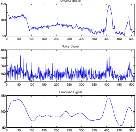
b. Test Case #2

The test case considers another general one

dimension signal original signal used to create

a noisy signal by adding AWGN and Rayleigh noise of known variance. The noisy signal is denoised using the proposed filter to generate the denoised signal.

Fig. 1.4 shows the results of the complete process. In this case only AWGN noise was added to the original signal with zero mean and standard deviation equal to unity. The computed threshold for the denoised signal was 1.6715e+13 and the mean square error was 12.3609. Fig. 1.5 shows the mean square error for various values of noise standard deviation with AWGN noise only. Noise Mean is zero in each case. As shown the relation is linear as expected.

Figure 1.5: Test Case #2 (AWGN only)

0 50 100 150 200 250 300 350 400 450 500 50

100

150 Original Signal

0 50 100 150 200 250 300 350 400 450 500 0

100 200 300 400

Noisy Signal

0 50 100 150 200 250 300 350 400 450 500 50

100 150

Denoised Signal

0 100 200 300 400 500 600 700 800 900 1000 0

2 4 6 8 10 12x 10

4 _{MSE vs Standard Deviation for RAYLEIGH+AWGN}

M

ea

n

S

qu

ar

e

E

rr

or

0 50 100 150 200 250 300 350 400 450 500 0

50 100 150 200

Original Signal

0 50 100 150 200 250 300 350 400 450 500 0

100 200

300 Noisy Signal

0 50 100 150 200 250 300 350 400 450 500 0

50 100 150

(6)

International Journal of Research (IJR)

Figure 1.6: Test Case #2 (AWGN only) (MSE vs. Standard Deviation)

Now, we will create the noisy signal by adding

AWGN and Rayleigh noise of known variance. Fig. 1.7 shows the results of the complete process. In this case AWGN and Rayleigh noise were added to the original signal with zero mean and standard deviation equal to unity. The computed threshold for the denoised signal was 1.1144e+13 and the mean square error was 18.2465.

Figure 1.7: Test Case #2 (AWGN + Rayleigh)

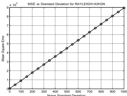
Fig. 1.8 shows the mean square error for various values of noise standard deviation with AWGN + Rayleigh. Noise Mean is zero in each case. As shown the relation is linear as expected.

Figure 1.8: Test Case #2 (AWGN + Rayleigh) (MSE vs. Standard Deviation)

As seen from both the results obtained (with AWGN only, and AWGN + Rayleigh) we can see that the increase in the noise level will increase the mean square error. The mean

square error is calculated between the original

and the denoised signal. As the Rayleigh noise

would degrade the originalsignalmore than

AWGN alone, the mean square error would be more in former case. The obtained results illustrate this fact.

c. Test Case #3

The test case considers a noisy ECG signal

generated using in-built Matlab data file (noisyecg.mat). This in-built noisy ECG signalhas a baseline shift and therefore does not represent the true amplitude. In order to remove the trend, a low order polynomial is

fitted to the noisy ECG signaland that

polynomial isthen used to de-trend it. This doesn’t removes any noise, but only remove the base line wander. As the noise is already added, so there is no need to re-add noise to this signal. The noisy ECG signal is further denoised using the proposed filter to generate the denoised signal.

0 100 200 300 400 500 600 700 800 900 1000 0

50 100 150 200

250 MSE vs Standard Deviation for AWGN

M

ea

n

S

qu

ar

e

E

rro

r

0 50 100 150 200 250 300 350 400 450 500 0

50 100 150

200 Original Signal

0 50 100 150 200 250 300 350 400 450 500 -200

0 200 400 600

Noisy Signal

0 50 100 150 200 250 300 350 400 450 500 0

50 100 150 200

Denoised Signal

0 100 200 300 400 500 600 700 800 900 1000 0

1 2 3 4 5 6 7 8 9x 10

4 _{MSE vs Standard Deviation for RAYLEIGH+AWGN}

M

ea

n

S

qu

ar

e

E

rro

(7)

International Journal of Research (IJR)

Figure 1.9: Test Case #3

Fig. 1.9 shows the results of the complete process. The computed threshold for the denoised signal was 2.8528e+15 and the mean square error was 0.1030.

8. Comparison

A smaller MSE implies a shorter transient duration. The notch filter given in [10] with time varying radius achieves an MSE of 0.12 while the traditional notch filter obtains an MSE of 0.2. The filter proposed in this work achieves an MSE of 0.10. Hence, it is clear that the proposed notch filter is effective in reducing transient response compared to traditional filters. It is also worth noting that higher order filters achieve lower MSE at the cost of increase in processing power and complexity.

Table 1.1: MSE Comparison

Filter

[10] Filter[11]

Traditional Filter

Proposed Filter

MSE 0.12 0.35 0.2 0.10

ConclusionECG is a measure of electrical activity of the heart over time. The signal is measured by electrodes attached to the skin and is sensitive to disturbances such as power source interference and noises due to movement artifacts. ECG of a patient is observed visually in time dominion. But examining the ECG curve visually is typically

inadequate. Signal processing approaches are performed to observe the ECG curve correctly. Frequency domain approaches, spectrum approximation and filtering are necessary to examine the ECG curve.

This work used a wavelet based window FIR filter that combined the discrete wavelet transform and two level FIR filter, each of which has its own characteristics and benefits. The proposed system resembles a new family of dyadic wavelet tight frames based on two scaling purposes and four distinct wavelets. One pair of the four wavelets are designed to be offset from the other pair of wavelets so that the integer transforms of one wavelet pair fall midway between the integer translates of the other pair.

Simultaneously, one pair of wavelets are designed to be approximate Hilbert transforms of the other pair of wavelets so that two complex (approximately analytic) wavelets can be formed. Therefore, they can be used to implement complex and directional wavelet transforms. This work developed a design procedure to obtain finite impulse response (FIR) filters that satisfy the numerous constraints imposed. This design procedure employed a fractional-delay all pass filter, spectral factorization, and filter bank completion. The simulation results show considerable performance enhancements with high degree of smoothness. Comparison based on mean square error, with previous work shows significant improvement in the noise reduction using proposed filter.

References

[1] H. B. Barlow, “Possible principles underlying the transformation of sensory

messages,” in in Sensory Communication,

1961.

[2] O. Sayadi and M. B. Shamsollahi, “Multiadaptive bionic wavelet transform: Application to ECG denoising and

baseline wandering reduction,” EURASIP

(8)

International Journal of Research (IJR)

Processing, vol. 2007, no. 1, p. 041274, 2007.

[3] G. Clifford, L. Tarassenko and N. Townsend, “One-pass training of optimal

architecture auto-associative neural

network for detecting ectopic beats,”

Electronics Letters, vol. 37, no. 18, pp. 1126-1127, 2001.

[4] P. C. Teo and D. J. Heeger, “Perceptual image distortion,” in in Proc. SPIE, 1994.

[5] R. Mark, P. Schluter, G. Moody, P. Devlin and D. Chernoff, “An annotated ECG

database for evaluating arrhythmia

detectors,” in IEEE Transactions on

Biomedical Engineering, 1982.

[6] N. Damera-Venkata, T. Kite, W. Geisler, B. Evans and A. Bovik, “Image quality assessment based on a degradation

model,” Image Processing, IEEE

Transactions on, vol. 9, no. 4, pp. 636-650, Apr 2000.

[7] D. L. Donoho, “De-noising by

soft-thresholding,” Information Theory, IEEE

Transactions on, vol. 41, no. 3, pp. 613-627, 1995.

[8] S. Jagtap, M. Chavan, R. Wagvekar and M. Uplane, “Application of the digital

filter for noise reduction in

electrocardiogram,” Journal of

Instrumentation, vol. 40, no. 2, pp. 83-86, 2010.

[9] G. Strang and T. Nguyen, Wavelets and Filter Banks, Wellesley College, 1996.

[10] R. Rajagopalan and A. Dahlstrom, “A Pole Radius Varying Notch Filter with

Transient Suppression for

Electrocardiogram,” International Journal

of Medical, Health, Pharmaceutical and Biomedical Engineering, vol. 8, no. 3, 2014.

[11] L. Tan, J. Jiang and L. Wang, “Pole-radius-varying IIR notch filter with

transient suppression,” Instrumentation

and Measurement, IEEE Transactions on,