R E S E A R C H
Open Access
The method of finding solutions of partial
dynamic equations on time scales
Hsuan-Ku Liu
**Correspondence:
[email protected] Department of Mathematics and Information Education, National Taipei University of Education, Taipei, Taiwan
Abstract
On time scales, one area lacking of development is the method of finding solutions on partial dynamic equations. This paper proposes a method for finding the exact solution of linear partial dynamic equations on arbitrage time scales. We modify the variational iteration method onRto find an approximation of the nonlinear partial dynamic equation onqN. As an example, the modified variational iteration method is applied toq-Berger equations and toq-Fisher equations. Their numerical results reveal that the proposed method is very effective.
Keywords: partial dynamic equations on time scales; nonlinearq-difference equation; variational iterative method; approximate solutions
1 Introduction
A time scale is a nonempty closed subset of real numbers. On time scale calculus, no-tations and theorems have been well established for the univariate case []. Solutions of ordinary differential equations, such as initial value problems and boundary value prob-lems, have been studied and published during the past two decades on time scales. In recent years, Hoffacker [] and Ahlbrandt and Morian [] demonstrated the related ideas to the multivariate case and studied partial dynamic equations on time scales. Notations and definitions on multivariate time scales calculus can be found in Bohner and Guseinov [, ]. Jackson [] extended the existing ideas of the time scales calculus [] to the mul-tivariate case. The method of generalized Laplace transform on time scales is applied to find solutions of the homogeneous and nonhomogeneous heat and wave equations. Re-cent developments in the method of finding solutions have aroused further interest in the discussion of partial dynamic equations on time scales.
For the nonlinear cases, methods of finding solutions are not mentioned for partial dy-namic equations on time scales. One of the difficulties for developing a theory of series solutions to nonlinear equations on time scales is that the formula for multiplications of two generalized polynomials is not easily found. If a time scale has constant graininess, Haile and Hall [] provided an exact formula for the multiplication of two generalized polynomials. Using the obtained results, the series solutions for linear dynamic equations are proposed on the time scalesRandT=hZ(difference equations with step sizeh). On generalized time scales, Mozyrska and Pawtuszewicz [] presented a formula for the mul-tiplication of generalized polynomials of degree one and degreen∈N. Liu [] provided a product rule of two generalized polynomials on the time scaleqZ={qn|n∈N} ∪ {}.
The variational iteration method proposed by He [] is a powerful mathematical tool in analyzing the nonlinear problems onR(the set of real numbers). Over the last few years, the variational iteration method (VIM) has been widely applied to analyze the nonlinear boundary value problems [], the nonlinear heat diffusion equations [] and the nonlin-ear reaction-diffusion equations []. An advantage of the VIM is that there is no need to make the assumption of the small parameters. On nonlinear partial dynamic equations, approximate solutions obtained by the variational iteration method are not found yet.
In this paper, we first explore a simple method to find the exact solution of linear partial dynamic equations on time scales. For the nonlinear cases, we derive a product rule of two generalized polynomials onqZ, which provides an idea for developing a series solutions on q-calculus. Applying the product rules, we extend the variational iteration method from the set of real numbersRto the time scalesqZ. The extension provides a method to find an approximate solution on the nonlinear partial dynamic equation onqZ. Moreover, the VIM is applied to find an approximation of theq-Berger equation and theq-Fisher equa-tion. By the numerical results, we found that the modified VIM is very effective. The VIM can be applied to other time scales when the multiplication rule of two generalized poly-nomials on these time scales is obtained.
This paper is organized as follows. In Section , the basic ideas of partial dynamic equa-tions on time scales are introduced. In Section , a method is explored to find an exact solution of linear initial value problems on time scales. In Section , a product rule of two generalized polynomials at is derived onqZand the variational iteration method is ap-plied to find an approximate solution of the Burger equation and the Fisher equation. In Section , numerical examples reveal that the proposed method is very effective. Finally, a concise conclusion and future directions are provided in Section .
2 Basic concepts on time scales
A time scale is an arbitrary nonempty closed subset of the real numbers. The calculus of time scales was introduced by Hilger [] in order to create a theory that can unify discrete and continuous analysis.
2.1 An introduction to time scales
In this subsection, we first define the forward and backward jump operators on time scales and then introduce the delta derivative and the integration.
Definition LetTbe a time scale. Fort∈Tthe forward jump operatorσ:T→Tis defined by
σ(t) :=inf{s>t|s∈T}
and the backward jump operatorρ:T→Tis defined by
ρ(t) :=sup{s<t|s∈T}.
The gain functionμ:T→[,∞) is defined by
According to the forward jump operator and the gain function, the delta derivative on the time scaleTis given as follows.
Definition Assume thatf :T→Ris a function and lett∈T. Ifσ(t) >t, the delta deriva-tive off(t) atton the time scaleTis defined as
fΔ(t) =f(σ(t)) –f(t)
μ(t) .
A functionf(t) onTis said to be differentiable attif its derivative exists att,∀t∈T.
Integration on a time scale can be viewed as an anti-derivative.
Definition If we have delta derivativeg(t) =fΔ(t) on the time scaleT, then the
anti-derivative is
f(t) = t
a
g(s)Δs+ constant, a,t∈T
and the definite integral on the time scaleTfollows as
b
a
g(s)Δs=f(b) –f(a), a,b∈T.
Following the delta derivative and integration, we define the generalized polynomials as follows.
Definition On the time scaleT, the generalized polynomialshk(·,t) :T→Rare
de-fined recursively as follows:
h(t,s) = , hk+(t,s) =
t
s
hk(τ,s)Δτ.
Hence, for each fixeds, the delta derivative ofhkwith respect totsatisfies
hΔkj(t, ) =
hk–j(t, ) ifk≥j,
ifk<j.
2.2 An introduction toq-calculus
Let
qN=qn|n∈N and qN=qN∪ {},
whereNdenotes the set of positive integers.
Ifaandqare real numbers such that <q< , then theq-shift factorial [] is defined by
(a;q)= and (a;q)n= n–
k=
–aqk, n∈N.
Definition Assume thatf :qN→Ris a function andt∈qN. Theq-derivative [] attis defined by
fΔ(t) =f(qt) –f(t) (q– )t , t=
and
fΔ() = lim
n→∞
f(qn) –f()
qn .
By computing the recurrence relation, theq-polynomials are represented as
hk(t,s) = k–
ν=
t–sqν ν
j=qj
onqN[].
Aq-difference equation is an equation that containsq-derivatives of a function defined onqN.
2.3 Multivariable calculus on time scales
The differentiation and integrations are introduced for functions of two variables on time scales []. Definitions on multivariate calculus on time scales can be found in Bohner and Guseinov [, ]. Following the line of ideas, the dynamic equations on time scales are extended to partial dynamic equations on time scales [, , ].
LetTandTbe any two time scales. Consider the ‘rectangle’T=T×T. For anyt∈T,
the jump operator oft= (t,t) fort∈Tandt∈Tis given as follows:
. The forward jump operatorsσ:T→Tbyσ(t) = (σ(t),σ(t))are defined as σ(t) =inf(s∈T|s>t)andσ(t) =inf(s∈T|s>t).
. The backward jump operatorsτ:T→Tbyτ(t) = (τ(t),τ(t))are defined as τ(t) =sup(s∈T|s<t)andτ(t) =sup(s∈T|s<t).
To use the notations for partial derivatives with respect to time scale variablestandt,
respectively, we employ lexicographic ordering for consistency. LetfΔ denote the time scale partial derivative with respect totand letfΔdenote the time scale partial derivative
with respect tot. Definitions of these partial derivatives are given as below [, ].
Definition Letf be a real-valued function onT. At (t,t)∈T=T×Twe sayf has a Δ-partial derivativefΔ(t,t) if for eachε> , there exists a neighborhoodUoft, with
U= (t–δ,t+δ)∩Tforδ> , such that
fσ(t),t
–f(s,t) –fΔ(t,t)
σ(t) –s≤σ(t) –s
for alls∈U. On the other hand, we sayf has aΔ-partial derivativefΔ(t,t) if for each ε> , there exists a neighborhoodVoft, withV= (t–δ,t+δ)∩Tforδ> , such that
ft,σ(t)
–f(t,s) –fΔ(t,t)
σ(t) –s≤σ(t) –s
Using the ideas of time scale partial derivatives, notations of mixed partial and high order partial derivatives are given as follows:
. fΔij(t)(if this value exists) denotes first taking the partial derivative with respect to tiand then taking the partial derivative with respect totj, so thatfΔij= (fΔi)Δj,
i,j= , .
. fΔni(t)(if this value exists) denotes taking the partial derivative off(t)with respect
totintimes.
The details and examples can be found in [] and [].
3 The exact solution of linear initial value problems on time scales
Lethk(t, ) andgk(t, ) be the generalized polynomials onTandT, respectively. In this
section, the variational iteration method onRis extended to provide a method of find-ing the exact solution of linear partial dynamic equations on time scales. The introduc-tion and the details of the variaintroduc-tional iteraintroduc-tion method can be found in the Appendix and in [].
3.1 The exact solution of the first-order linear partial dynamic equations
We first consider the first-order linear partial dynamic equations as the form
uΔ=cuΔ onT
×T,
u(,t) =f(t) onT,
()
wheref(t) = Ki=aigi(t, ) onTandai,i= , . . . ,Kare real numbers.
The basic character of the variational iteration method is to construct a correction func-tional for the system, which reads
un+(t,t) =un(t,t) +
t
t
λLun(s,t) +Nu˜n(s,t)
Δs,
whereLis a linear operator onT,Nis a linear (or nonlinear) operator onT(orT×T), λis a Lagrange multiplier which can be identified optimally by variational theory,unis the
nth approximation, andu˜ndenotes a restricted variation, that is,δu˜n= .
The linear operatorLis selected as
Lu=uΔ
and the other operatorNis selected as
Nu= –cuΔ.
Make the above correction functional stationary with respect toun
δun+(t,t) =δun(t,t) +δ
t
λuΔ(s,t
) +Nu˜n(s,t)
Δs
= +λ(t)
δun(t,t) +
t
λΔ(s)δun
σ(s),t
We, therefore, have the following stationary conditions:
+λ(t) = ,
λΔ(s) = .
The Lagrange multiplier can be readily identified
λ(s) = –.
As a result, the variational iteration formula is obtained
un+(t,t) =un(t,t) –
t
uΔ
n (s,t) +Nun(s,t)
Δs. ()
Using the initial conditionu=f(t) and the iteration formula (), we have the following
equations:
u(t,t) =f(t) –
t
fΔ(t
)Δs
=f(t) +cfΔ(t)h(t, ),
u(t,t) =u(t,t) –
t
cfΔ(t
)h(s, )Δs
=u(t,t) +cfΔ
(t
)h(t, )
=f(t) +cfΔ(t)h(t, ) +cfΔ
(t)h(t, )
and
uk(t,t) = k
j=
cjfΔj(t
)hj(t, ).
Askis large enough such thatfΔkequals to zero, the series solutionukis the exact solution of ().
Example Consider the initial value problem
uΔ=cuΔ onT
×T,
u(,t) =gk(t, ) onT,
()
wheregk(t, ) is a generalized polynomial onT. The function
uk(t,t) = k
j=
cjgk–j(t, )hj(t, )
Proof We now verify that the obtained functionukactually solves the initial value problem
(). First, we show that the obtained function satisfies the initial condition. Sinceh(t,s)≡
for allt,sandhj(, )≡ forj> , we have
uk(,t) =gk(t, ).
Second, we display the obtained functionuksatisfying the equation by
uΔ
k (t,t) = k
j=
cjgk–j(t, )hj–(t, ),
cuΔ
k (t,t) = k–
j=
c(j+)gk–j–(t, )hj(t, ) = k
j=
cjgk–j(t, )hj–(t, ).
This implies thatuΔ
k (t,t) –cu
Δ
k (t,t) = onT×T.
3.2 The exact solution of the second-order linear partial dynamic equations
Consider the second-order partial dynamic equation as the form
uΔ=cuΔ onT
×T,
u(,t) =f(t) onT,
()
wheref(t) = Ki=aigi(t, ) onTandai,i= , . . . ,Kare real numbers.
In this work, the linear operatorLis selected as
Lu=uΔ
and the other operatorNis selected as
Nu= –cuΔ.
Using the initial conditionu(t,t) =f(t) and the iteration formula (), we have the
following equations:
u(t,t) =f(t) –
t
cfΔ(t
)Δs
=f(t) +cfΔ
(t)h(t, ),
u(t,t) =u(t,t) –
t
cfΔ(t
)h(s, )Δs
=u(t,t) +fΔ
(t)h(t, )
=f(t) +cfΔ
(t)h(t, ) +cfΔ(t)h(t, )
and
uk(t,t) = k
j=
As k is large enough such thatfΔ(k) equals to zero, the series solutionu
k is the exact
solution of ().
Example Consider the IVP
uΔ=cuΔ onT
×T,
u(,t) =gk(t, ) onT,
()
wheregk(t, ) is a generalized polynomial ofT. The function
uk/(t,t) =
k/
j=
cjgk–j(t, )hj(t, )
is the exact solution of ().
The exact solution of Example is also obtained by Jackson []. He transformed the IVP into an ODE and obtained the exact solution as
u(t,t) =
k/
j=
cjgk–j(t, )hj(t, ),
wherek/denotes the floor ofk/.
When the initial condition can be represented as a finite series of generalized polyno-mials, we have proposed a useful method of finding the exact solution of partial dynamic equations on time scales. When the initial condition is represented as an infinite series of generalized polynomials, the approximate solution can be obtained by the same man-ner. In the following section, we consider the nonlinear partial dynamic equation on the specific time scales.
4 Approximation solutions of nonlinearq-partial dynamic equations
In this section, we extend the variational iteration method to find an approximate solution of nonlinear initial value problems on the time scaleqN.
To extend the variational iteration method, we first display a production rule [] of two q-polynomials at which will be used to derive an approximate solution in the following discussion.
Theorem Let hi(t, )and hj(t, )be two q-polynomials at zero.We have
hi(t, )hj(t, ) =
(qi+;q) j
(q;q)j
hi+j(t, ).
Proof Since
hi+j(t, ) = i+j–
ν=
t
ν μ=qμ
we have
Proof It suffices to show that
(qi+;q)
Lethkandgkbe generalized polynomials ofqN andqN. The variational iteration method
is now applied to find an approximate solution of the nonlinear partial dynamic equations as the form
uΔ=Nu onqN
×qN,
u(,t) =gk(t, ) onqN.
When the linear operatorLis selected as
and the other operatorNis selected as –Nu, the variational iteration formula is obtained
Example Consider the partial dynamic equations as the form
uΔ=uuΔ onT
×T,
u(,t) =gk(t, ) onT.
With the variational iteration formula, we obtain the first few components ofun(t,t):
u(t,t) =u(t,t) –
In the same manner, the rest of components of the iteration formula are obtained itera-tively.
4.1 Applications to theq-Burger equation and the Fisher equation
q-Burger equation
First of all, we consider theq-Burger equation as the form
uΔ–uuΔ–αuΔ= onqN
×qN,
When the linear operator and the nonlinear operator are selected asLu=uΔand –Nu= –uuΔ–αuΔ, respectively, the variational iteration formula is obtained as
un+(t,t) =un(t,t) –
In the same manner, the rest of components of the iteration formula are obtained itera-tively.
q-Fisher equation
Secondly, we consider theq-Fisher equation, which is a nonlinear reaction diffusion equa-tion, as the form
uΔ–αuΔ–βu( –u) = onqN
×qN,
The variational iteration formula is obtained as
In the same manner, the rest of components of the iteration formula are obtained itera-tively.
5 Numerical results
The approximate solutions introduced in the previous sections will be illustrated with some examples.
Let T=T= .N={., ., ., . . . , }, where is the cluster point of qN. The
q-shift factorial withq= . is given as
and theq-polynomials are represented as
hk(t, ) = k–
ν=
t
ν
j=.j
= t
k
k–
ν=
ν
j=.j
= t
k
k–
ν=( – .ν)
,
t∈ {.n,n∈N} ∪ {}andh
k(, ) = . The multiplication of two generalized polynomials
hk(t, ) andhl(t, ) is obtained as
hk(t, )hl(t, ) =H(k,l)hk+l(t, ),
whereH(k,l) = (.k+;.)l
(.;.)l . For example,H(, ) =
(.;.)
(.;.) =
(–.) (–.) =
. .= ..
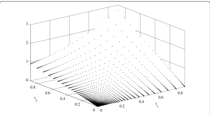
Example Consider the nonlinear partial dynamic equation as the form
uΔ–uuΔ–uΔ= on .N×.N, u(,t) =g(t, ) on .N.
()
The initial approximation can be given as
u(t,t) =g(t, )
according to the initial condition. By the variational iteration formula (), the first two components ofun(t,t) are obtained:
u(t,t) =
+h(t, )
g(t, ),
u(t,t) =
+h(t, ) + h(t, ) + .h(t, )
g(t, ).
The rest of components of the iteration formula are obtained in the same manner. The responses ofu(t,t) are shown in Figure .
Example Consider the Fisher equation as the form
uΔ–uΔ–u( –u) = on .N×.N,
u(,t) =g(t, ) on .N.
()
With the initial conditionu(t,t) =g(t, ), the first two components are obtained
u(t,t) =g(t, ) +
g(t, ) – .g(t, )
(t, ) =g(t, ) +G(t)g(t, ),
u(t,t) =g(t, ) +G(t)h(t, ) +
gΔ(t) +G(t) – G(t)g(t, )h(t, )
–g(t)H(, )h(t, )
=g(t, ) +
g(t, ) – .g(t, )
h(t, )
+–. +g(t, ) – .g(t, ) –
g(t, ) – .g(t, )
g(t, )
h(t, )
– .g(t, ) – .g(t, )
h(t, )
=g(t, ) +
g(t, ) – .g(t, )
h(t, )
+–. +g(t, ) – .g(t, ) + .g(t, )
h(t, )
– ..g(t, ) – .g(t, ) + .g(t, )
h(t, ),
whereG(t) =g(t, ) – .g(t, ). The rest of components of the iteration formula are
obtained in the same manner. The responses ofu(t,t) are shown in Figure .
Now, we have demonstrated a method for finding an approximate solution of nonlinear partial dynamic equations onqN ×qN. The proposed tool could also be applied to other nonlinearq-partial dynamic equations.
In future studies, we intend to derive the multiplication rule of two generalized polyno-mials and extend the application of the variational iteration method to nonlinear partial dynamic equations on other time scales.
6 Conclusion and future direction
In this paper, we have propose a method to find the exact solution of the linear partial dynamic equation on time scales and to find an approximate solution of the nonlinear q-partial dynamic equations. Moreover, this method is applied to provide an approximate solution of theq-Berger equations and theq-Fisher equations.
To extend the method to other time scales, it is important to derive a multiplication rule of two generalized polynomials on the other time scales. On the other hand, approximate solutions as well as their properties of the nonlinear partial dynamic equations, such as Benjamin-Ono equations and the Benjamin-Bona-Mahony equations, are not found on qNyet. In the future studies, we would intend to derive the multiplication rule of two gen-eralized polynomials or to provide an approximation of other nonlinearq-partial dynamic equations by using the proposing method.
Appendix: Basic ideas of the variational iteration method
To clarify the ideas of the variational iteration method, we consider the following nonlinear equation:
Lu(t) +Nu(t) =g(t),
whereLis a linear operator,Nis a nonlinear operator andgis an inhomogeneous term. According to the variational iteration method, we can construct a correction functional as follows:
un+(t) =un(t) +
t
λLun(s) +Nu˜n(s) –g(s)
ds,
where λis a general Lagrange multiplier, uis an initial approximation which must be
chosen suitably andu˜nis considered as a restricted variation, that is,δu˜n= . To find the
optimal value ofλ, we make the above correction functional stationary with respect toun,
noticing thatδun() = , and have
δun+(t) =δun(t) +δ
t
λLun(s)ds= .
Having obtained the optimal Lagrange multiplier, the successive approximationsun,n≥,
of the solutionuare determined upon the initial functionu. Therefore, the exact solution
is obtained at the limit of the resulting successive approximations.
Competing interests
The author declares that they have no competing interests.
Received: 14 November 2012 Accepted: 30 April 2013 Published: 17 May 2013 References
1. Bohner, M, Peterson, A: Dynamic Equations on Time Scales: An Introduction with Applications. Birkhäuser, Boston (2001)
2. Hoffacker, J: Basic partial dynamic equations on time scales. J. Differ. Equ. Appl.8, 307-319 (2002) (in honor of Professor Lynn Erbe)
3. Ahlbrandt, CD, Morian, C: Partial differential equations on time scales. J. Comput. Appl. Math.141, 35-55 (2002) 4. Bohner, M, Guseinov, GS: Partial differentiation on time scales. Dyn. Syst. Appl.13, 351-379 (2004)
6. Jackson, B: Partial dynamic equations on time scales. J. Comput. Appl. Math.186, 391-415 (2006)
7. Haile, BD, Hall, LM: Polynomial and series solutions of dynamic equations on time scales. Dyn. Syst. Appl.12, 149-157 (2003)
8. Mozyrska, D, Pawtuszewicz, E: Hermite’s equations on time scales. Appl. Math. Lett.22, 1217-1219 (2009) 9. Liu, H-K: The formula for the multiplicity of two generalized polynomials on the time scale. Appl. Math. Lett.25,
1420-1425 (2012)
10. He, J-H: Variational iteration method - some recent results and new interpretations. J. Comput. Appl. Math.207, 3-17 (2007)
11. Momani, S, Abusasd, S, Odibat, Z: Variational iteration method for solving nonlinear boundary value problems. Appl. Math. Comput.183, 1351-1358 (2006)
12. Ganji, DD, Afrouzi, GA, Talarposhti, RA: Application of variational iteration method and homotopy-perturbation method for nonlinear heat diffusion and heat transfer equations. Phys. Lett. A368, 450-457 (2007)
13. Ganji, DD, Afrouzi, GA, Talarposhtib, RA: Application of He’s variational iteration method for solving the reaction-diffusion equation with ecological parameters. Comput. Math. Appl.54, 1010-1017 (2007)
14. Hilger, S: Analysis on measure chains - a unified approach to continuous and discrete calculus. Results Math.18, 18-56 (1990)
15. Koornwinder, TH:q-special functions: a tutorial. arXiv:math/9403216v1
doi:10.1186/1687-1847-2013-141