Vieta Pell and Vieta Pell Lucas polynomials

(1)

R E S E A R C H

Open Access

Vieta-Pell and Vieta-Pell-Lucas polynomials

Dursun Tasci and Feyza Yalcin

*

*_{Correspondence:}

[email protected] Department of Mathematics, Faculty of Science, Gazi University, Ankara, 06500, Turkey

Abstract

In the present paper, we introduce the recurrence relation of Vieta-Pell and Vieta-Pell-Lucas polynomials. We obtain the Binet form and generating functions of Vieta-Pell and Vieta-Pell-Lucas polynomials and define their associated sequences. Moreover, we present some differentiation rules and finite summation formulas. MSC: Primary 11C08; secondary 11B39

Keywords: Vieta-Pell; Vieta-Pell-Lucas polynomials

1 Introduction

Andre-Jeannin [] introduced a class of polynomialsUn(p,q;x) deﬁned by

Un(p,q;x) = (x+p)Un–(p,q;x) –qUn–(p,q;x), n≥, with the initial valuesU(p,q;x) =  andU(p,q;x) = .

Lucas polynomials were studied as Vieta polynomials by Robbins []. Vieta-Fibonacci and Vieta-Lucas polynomials are deﬁned by

Vn(x) =xVn–(x) –Vn–(x), n≥, vn(x) =xvn–(x) –vn–(x), n≥,

respectively, whereV(x) = ,V(x) =  andv(x) = ,v(x) =x[]. The recursive properties of Vieta-Fibonacci and Vieta-Lucas polynomials were given by Horadam [].

Forp=  andq= , Vieta-Fibonacci polynomials are a special case of the polynomials

Un(p,q;x) in []. Further,Un,m(p,q;x) in [] forp= ,q= ,m=  gives Vieta-Fibonacci

polynomials.

Chebyshev polynomials are a sequence of orthogonal polynomials which can be deﬁned recursively. Recall that thenth Chebyshev polynomials of the ﬁrst kind and second kind are denoted byTn(x) andUn(x), respectively.

It is well known that the Chebyshev polynomials of the first kind and second kind are closely related to Vieta-Fibonacci and Vieta-Lucas polynomials. So, in [] Vitula and Slota redefined Vieta polynomials as modified Chebyshev polynomials. The related features of Vieta and Chebyshev polynomials are given as

Vn(x) =Un

 x

[],

vn(x) = Tn



x see [, ]

.

(2)

For|x|> , we considertn(x) andsn(x) polynomials by the following recurrence relations:

tn(x) = xtn–(x) –tn–(x), n≥, sn(x) = xsn–(x) –sn–(x), n≥,

wheret(x) = ,t(x) =  ands(x) = ,s(x) = x. We calltn(x) thenth Vieta-Pell

polyno-mial andsn(x) thenth Vieta-Pell-Lucas polynomial.

The relations below are obvious

sn(x) = Tn(x),

tn+(x) =Un(x).

The ﬁrst few terms oftn(x) andsn(x) are as follows:

t(x) = x, s(x) = x– , t(x) = x– , s(x) = x– x, t(x) = x– x, s(x) = x– x+ , t(x) = x– x+ , s(x) = x– x+ x, t(x) = x– x+ x, s(x) = x– x+ x– , t(x) = x– x+ x– , s(x) = x– x+ x– x.

The aim of this paper is to determine the recursive key features of Pell and Vieta-Pell-Lucas polynomials. In conjunction with these properties, we examine their interrela-tions and deﬁne their associated sequences. Furthermore, we present some diﬀerentiation rules and summation formulas.

2 Main results

Some fundamental recursive properties of Vieta-Pell and Vieta Pell-Lucas polynomials are given in this section.

Characteristic equation

Vieta-Pell and Vieta-Pell-Lucas polynomials have the following characteristic equation:

λ– xλ+  =  with the rootsαandβ

α=x+√x_{– ,}

β=x–√x_{– .}

Also,αandβsatisfy the following equations:

α+β= x,

αβ= , ()

(3)

Binet form

By appropriate procedure, we can easily ﬁnd the Binet forms as

tn(x) =

αn_–_βn

α–β , ()

sn(x) =αn+βn. ()

Generating function

Vieta-Pell and Vieta-Pell-Lucas polynomials can be deﬁned by the following generating functions:

∞

n=

tn(x)yn=y

 – xy+y–,

∞

n=

sn(x)yn= ( – xy)

 – xy+y–.

Negative subscript

We can also extend the deﬁnition oftn(x) andsn(x) to the negative index

t–n(x) = –tn(x),

s–n(x) =sn(x).

Simson formulas

tn+(x)tn–(x) –tn(x) = –,

sn+(x)sn–(x) –sn(x) = 

x– .

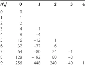
We arrange the ﬁrst ten coeﬃcients oftn(x) in Table . LetT(n,j) denote the element in

rownand columnj, wherej≥,n≥. As seen from the Table , it is obvious that

T(n, ) = T(n– , ) +T(n– , )

Table 1 The ﬁrst ten coefﬁcients oftn(x)

n\j     

0 0

1 1

2 2

3 4 –1

4 8 –4

5 16 –12 1

6 32 –32 6

7 64 –80 24 –1

8 128 –192 80 –8

(4)

can be written like the coeﬃcients of Pell polynomials in []. Moreover,

n– 

j=

T(n,j) =n.

For example, forn=  we can ﬁnd 

j=

T(,j) =T(, ) +T(, ) +T(, ) +T(, ) = .

LetPndenote thenth Pell number, so we have

n– 

j=

T(n,j)=Pn.

2.1 Interrelations oftn(x) andsn(x)

Most of the equations below can be obtained by using the Binet form and convenient routine operations

tn+(x) –tn–(x) =sn(x) = xtn(x) – tn–(x), () sn+(x) –sn–(x) = 

x– tn(x), ()

tn(x)sn(x) =tn(x),

s_n(x) + x– t_n(x) = sn(x),

s_n(x) – x– t_n(x) = ,

t_n_+(x) –t_n(x) =tn+(x),

s_n_+(x) –s_n(x) = x– tn+(x), s_n_+(x) +s_n(x) = xsn+(x) + , t_n_+(x) –t_n_–(x) = xtn(x),

sn(x)sn+(x) – 

x– tn(x)tn+(x) = x, sn(x)sn+(x) + 

x– tn(x)tn+(x) = sn+(x), sn(x) –  = 

x– t__n(x),

tn+(x) –xtn(x) =

 sn(x), sn+(x) – xsn(x) = 

x– tn(x).

Proposition  sn(x– ) –sn(x) = –.

Proof Consider the expressionsn(x– ). Thenα,β,Δare replaced byα∗,β∗,Δ∗,

re-spectively. So,α∗=α,β∗=β,Δ∗= xΔand by using the Binet form, the proof is

(5)

2.2 Associated sequences

applied repeatedly, the results emerge

t_nj(x) =s_n(j–)(x) =Δjtn(x),

Since the derivation function ofsn(x) is a polynomial, all of the derivatives must exist for

(6)

Proposition 

In this section we deal with the matrix

V=

(7)

It is known that

If we use the matrix technique for summation in [], we get the ﬁrst ﬁnite summation as follows. be the series of matrices. Then we have

VA=V+V+· · ·+Vn–+Vn.

(8)

=(α+β) – αβ– (α

m+₊_βm+_{) +}_αβ₍_αm₊_βm₎

 – x

=x–  – (α

m+₊_βm+_{) +}_αm₊_βm

( –x)

by ()

=sm+(x) –sm(x) +  – x (x– )

by ().

This completes the proof.

Theorem  LetVbe a square matrix such thatV= xV–I.Then,for all n∈Z+_,

Vn=tn(x)V–tn–(x)I,

where tn(x)is the nth Vieta-Pell polynomial andIis a unit matrix.

Proof The proof is obvious from induction.

Competing interests

The authors declare that they have no competing interests.

Authors’ contributions

The authors declare that the research was realized in collaboration with the same responsibility and contributions. Both authors read and approved the ﬁnal manuscript.

Acknowledgements

The authors thank the referees for their valuable suggestions, which improved the standard of the paper.

Received: 4 April 2013 Accepted: 11 July 2013 Published: 24 July 2013

References

1. Andre-Jeannin, R: A note on general class of polynomials. Fibonacci Q.32(5), 445-454 (1994)

2. Robbins, N: Vieta’s triangular array and a related family of polynomials. Int. J. Math. Math. Sci.14, 239-244 (1991) 3. Horadam, AF: Vieta polynomials. Fibonacci Q.40(3), 223-232 (2002)

4. Djordjevic, GB: Some properties of a class of polynomials. Mat. Vesn.49, 265-271 (1997) 5. Vitula, R, Slota, D: On modiﬁed Chebyshev polynomials. J. Math. Anal. Appl.324, 321-343 (2006) 6. Jacobsthal, E: Über vertauschbare polynome. Math. Z.63, 244-276 (1955)

7. Halici, S: On the Pell polynomials. Appl. Math. Sci.5(37), 1833-1838 (2011)

8. Mahon, JM, Horadam, AF: Matrix and other summation techniques for Pell polynomials. Fibonacci Q.24(4), 290-309 (1986)

doi:10.1186/1687-1847-2013-224