R E S E A R C H
Open Access
Threshold dynamical analysis on a class of
age-structured tuberculosis model with
immigration of population
Lili Liu
1*, Xinzhi Ren
2and Zhen Jin
1*Correspondence: [email protected] 1Complex Systems Research Center, Shanxi University, Taiyuan, Shan’xi 030006, China
Full list of author information is available at the end of the article
Abstract
Some studies show that latency and relapse, especially the age-dependent latency and relapse, may affect the transmission dynamics of tuberculosis model. Meanwhile, the immigration of infected individuals induces the loss of disease-free steady state and hence no basic reproduction number. In our work, a class of age-structured tuberculosis model with immigration is proposed, where the new individuals can immigrate into the susceptible, latent, infectious and removed compartments. We show that the endemic steady state is unique and globally asymptotically stable by using the Lyapunov functional. Numerical simulations are given to support our theoretical results.
Keywords: tuberculosis model; age-structured; immigration; global stability; Lyapunov functional
1 Introduction
Tuberculosis (TB), mainly caused byMycobacterium tuberculosis, is a widespread infec-tious disease and has become a global public health issue. Despite various treatment strate-gies and beneficial policies on TB patients, the current global TB remains a leading cause of death from an infectious disease. According to reports, there were one death in five in England in the th century []. About .×cases of TB globally is estimated in ,
in which India has the largest total infected population, with an estimated . million new cases; China has the second largest TB epidemic, with more than .×new cases every
year [].
Mathematical models have been a useful tool to understand and analyze the transmis-sion dynamics of TB and other infectious diseases. In [], a SEI type of TB model with a general contact rate is considered, and the global stability of equilibria is derived. In [], a TB model with early and late latent stages is introduced to discuss effectiveness of treating TB patients at different stages. The reader can refer to more related mathematical models for TB; see [–]. It is well known that TB experiences a latent phase as well as a relapse phase which are the removed individuals who have been previously infected, but revert back to the infectious compartments due to the reactivation (see [, ]). Hence, in this paper, we focus on an SEIR-type model.
The level of infectiousness and the likelihood of progression may depend on the types of infectious diseases and individuals’ status. Thus, the age-structured epidemic models are thought to be more practical to describe certain disease features. Taking into consideration the age-dependent latency and relapse, Liu [] established and researched the following initial-boundary-value problem for a hybrid system of ordinary and partial differential equations:
⎧ ⎪ ⎪ ⎪ ⎪ ⎪ ⎨ ⎪ ⎪ ⎪ ⎪ ⎪ ⎩
dS(t)
dt =s–μsS(t) –βS(t)I(t),
(∂t∂ +∂a∂)e(t,a) = –σ(a)e(t,a) –μee(t,a),
dI(t) dt =
∞
σ(a)e(t,a)da– (μi+k)I(t) + ∞
γ(b)r(t,b)db,
(∂t∂ +∂b∂)r(t,b) = –γ(b)r(t,b) –μrr(t,b),
(.)
with the boundary conditions
e(t, ) =βS(t)I(t), r(t, ) =kI(t) (.)
fort≥ and the initial conditions
S() =S, e(,a) =e(a), I() =I, r(,b) =r(b) (.)
fora,b≥. This model can be used to describe TB transmission dynamics. The initial conditions satisfyS,I∈R+ande(a),r(b)∈L
+(R+,R+), whereL+(R+,R+) is the space
of functions on [,∞) that are nonnegative and Lebesgue integrable. Here,S(t) andI(t) are the densities of susceptible and infectious individuals at timet, ande(t,a) andr(t,b) rep-resent the densities of latent and removed individuals at timet, ageaandb, respectively.
aandbare referred to the latent age and the time spending at the removed compartment.
sdenotes the recruitment of susceptible individuals, μj(j=s,e,i,r) denotes their per
capita mortality rate andkdenotes the recovery rate.σ(a) andγ(b) are the removal rate from latent and removed compartments, respectively. The authors showed the asymptotic smoothness of solutions and uniform persistence of system (.). Furthermore, they ob-tained the basic reproduction number, which played as a threshold parameter and sat-isfied that if< , then the disease-free equilibrium of system (.) is locally and globally asymptotically stable, while if> , then the endemic equilibrium uniquely exists and it is locally and globally asymptotically stable. More related work is done to understand the dynamics of age-structured models; see [–]. Famous books on age-structured models are by Webb [], Iannelli [] and Smithet al.[].
immigration into the latent compartment. It is well known that the model will no longer have the disease-free equilibrium and the basic reproduction number, and there will al-ways have a unique endemic equilibrium which is globally asymptotically stable by using a global Lyapunov function. More related work can be found in [–] and references therein.
In this paper, we propose and investigate a TB model with immigration into the four compartments. We also incorporate into the continuous age-dependent in latent and re-moved compartments. It is a generalization of model proposed in []. According to math-ematical analysis, we show that TB always exists in a region and the endemic equilibrium is unique and globally asymptotically stable. This paper is organized as follows. In the next section, we will formulate the model. In Section , we show the mathematical well-posedness of our model. In Section , we investigate the asymptotic smoothness of the semi-flow generated by our model and the existence of compact attractor. In Section , we show our dynamics results, including the existence and global stability of the unique endemic steady state. Some simulations and conclusion are provided in Section and Sec-tion , respectively.
2 Model formulation
This section we devote to formulating our model.
Assume that there is constant recruitment into the susceptible and infectious compart-ments at ratessandi, respectively. The recruitment into the latent and removed
com-partments with age-in-classaandbtake place at rates denotede(a) andr(b),
respec-tively. The transfer diagram is shown in Figure . The corresponding hybrid system of ordinary and partial differential equations is the following form:
⎧ ⎪ ⎪ ⎪ ⎪ ⎪ ⎨ ⎪ ⎪ ⎪ ⎪ ⎪ ⎩
dS(t)
dt =s–μsS(t) –βS(t)I(t),
(∂ ∂t+
∂
∂a)e(t,a) =e(a) –σ(a)e(t,a) –μee(t,a), dI(t)
dt =i+ ∞
σ(a)e(t,a)da– (μi+k)I(t) + ∞
γ(b)r(t,b)db,
(∂ ∂t+
∂
∂b)r(t,b) =r(b) –γ(b)r(t,b) –μrr(t,b),
(.)
with the boundary conditions
e(t, ) =βS(t)I(t), r(t, ) =kI(t), t≥,
and the initial conditions
S() =S, e(,a) =e(a), I() =I, r(,b) =r(b), a,b≥.
Note that system (.) considers the immigration of all compartments, which is different from system (.), where only considers the immigration of susceptible compartment. All
Figure 1 The schematic flow diagram of our model.
Here, the terms [σE] and [γR] stand for0∞σ(a)e(t,a)da
parameters have the same biological meanings with system (.) and satisfy the following assumptions.
Assumption . Consider system (.), we assume that:
(A) All constant parameterss,i,μs,μe,μi,μr,k> .
(A) The functionsσ(a),γ(b)∈L∞(R+,R+), and denoteσinf, γinf and σsup,γsupas the essential infimums and the essential supremums ofσ andγ, respectively.
(A) σ(a)andγ(b)are Lipschitz continuous onR+with Lipschitz coefficientsMσandMγ, respectively.
(A) ∞
σ(a)da= and ∞
γ(b)db= . (A) e,r∈L(R+,R+), and denote¯e=
∞
e(a)da,¯r= ∞
r(b)db. (A) ¯e,¯r∈R+, and¯e+¯r> .
Define the space of functionsXasX=R+×L
+(R+,R+)×R+×L+(R+,R+) with the norm
(x,x,x,x)X=|x|+ ∞
x(a) da+|x|+ ∞
x(b) db.
Following the standard theory [], it can be verified that system (.) with initial-boundary conditions has a unique nonnegative solution for all time. Thus, there exists a continuous semi-flow associated with system (.), that is,:R+×X→Xtakes the
following form:
(t,x) =S(t),e(t,·),I(t),r(t,·), t≥,x∈X,
with
(t,x)X=S(t),e(t,·),I(t),r(t,·)X
= S(t) +
∞
e(t,a) da+ I(t) +
∞
r(t,b) db. (.)
3 The well-posedness of system (2.1)
This section is devoted to the positivity and boundedness of solutions. Assume that functionf(a,s) is continuous inR+×R+, then one has
t
a
f(a,s)ds da+
∞
t a
a–t
f(a,s)ds da=
∞
s+t
s
f(a,s)ds da, (.)
which is achieved by changing the order of integration in two double integrals. This will be useful in the later proofs.
For simplification, we denote
ε(a) =σ(a) +μe, ρe(a) =exp
–
a
ε(s)ds
, θe=
∞
σ(a)ρe(a)da,
η(b) =γ(b) +μr, ρr(b) =exp
–
b
η(s)ds
, θr=
∞
It follows from (A) of Assumption . that
Similar to [], solutions of the PDE parts are
e(t,a) =
Finally, we define the state space for system (.) as
=S(t),e(t,·),I(t),r(t,·)∈X:S(t) +
Proposition . Consider system(.),we have
(i) is positively invariant for,that is,(t,x)∈,for∀t≥andx∈;
(ii) is point dissipative andattracts all points inX.
Proof From (.), we have
d
Before calculating the derivative of semi-flow, we first show that
Note that the last term is obtained by using (.). Furthermore, letτ =t–aandτ=a–t
in the first and second integrals on the right-hand side of (.), respectively, one has
∞
Here, we put our main attentions on dealing with the last term. Following (.), we have
t
Applying (.) to replace the last term of (.), one gets
Similarly, one can obtain
d dt
∞
r(t,b)db=r(t, ) –
∞
η(b)r(t,b)db+¯r. (.)
Combining (.)-(.) and the first and third equations of (.) yields
d dt
S(t) +
∞
e(t,a)da+I(t) +
∞
r(t,b)db
= (s+¯e+i+¯r) –
μsS(t) +μe ∞
e(t,a)da+μiI(t) +μr ∞
r(t,b)db
≤∗–μ∗
S(t) +
∞
e(t,a)da+I(t) +
∞
r(t,b)db
,
which implies
(t,x)X≤
∗
μ∗ –e –μ∗t
∗
μ∗ –xX
, fort≥. (.)
Obviously,(t,x)∈holds true for any solution of (.) satisfyingx∈andt≥. Thus,is positively invariant for semi-flow{(t)}t≥.
Moreover, it follows from (.) thatlim supt→∞(t,x)X≤∗/μ∗ for anyx∈X. Therefore,is point dissipative andattracts all points inX. This completes the proof.
Combining Assumption . and Proposition ., we have the following two propositions.
Proposition . If x∈X andxX≤M for some constant M≥∗/μ∗,then the follow-ing statements hold true for t≥:
(i) ≤S(t),∞e(t,a)da,I(t),∞r(t,b)db≤M; (ii) e(t, )≤βM,r(t, )≤kM.
Proposition . Let B⊂X be bounded.Then (i) (R+,B)is bounded;
(ii) is eventually bounded onB;
(iii) ifM≥∗/μ∗is a bound forB,thenMis also a bound for(R+,B);
(iv) given anyL≥∗/μ∗,there existsT=T(B,M)such thatLis a bound for(t,B)
whenevert≥T.
Now, we give the following proposition on the asymptotic lower bounds for system (.).
Proposition . If x∈X,then
lim inf
t→∞ S(t)≥ms, lim inft→∞ I(t)≥mi,
lim inf
Proof It follows from the first equation of system (.) that
S=s–μsS–βSI≥s– (μs+βM)S,
which implies that
lim inf
t→∞ S(t)≥
s μs+βM
ms.
Similarly, one has
lim inf
t→∞ I(t)≥
i+ (σinf+γinf)M μi+k
mi.
Following (.), one can see that
lim inf
t→∞ e(t, ) =βSI≥βmsmime, lim inft→∞ r(t, ) =kI≥kmimr.
The proof is completed.
4 Asymptotic smoothness
In order to obtain global properties of the semi-flow{(t)}t≥, it is important to prove
that the semi-flow is asymptotically smooth. We introduce two definitions and a useful lemma.
Definition . A function Y :R→X is called a total trajectory of if Y satisfies
s(Y(t)) =Y(t+s) for allt∈Rands≥.
Definition . A non-empty invariant compact setAis called the compact attractor of a classBof sets ifdist((t,B),A)→ for eachB∈B, where
dist(t,B),A= sup
x∈t(B)
inf
y∈Ax–yX.
Remark . For any pointy∈A, it follows from Definitions . and ., and [], Theo-rem ., that there exists a total trajectoryY(·) withy() =yandy(t)∈Afor allt∈R.
Lemma . []Let D⊆R.For j= , ,suppose fj:D→Ris a bounded Lipshitz continu-ous function with bound Kjand Lipschitz coefficient Mj.Then the product function ffis Lipschitz with coefficient KM+KM.
In order to prove the asymptotic smoothness of the semi-flow, we will apply the follow-ing result, which is a special case of [], Theorem ..
Lemma . If the following two conditions hold for any bounded closed set B⊂X,then the semi-flow(t,x) =(t,x) +(t,x) :R+×X→X is asymptotically smooth in X.
(i) limt→∞diam(t,B) = ;
The following result is used to verify (ii) of Lemma ., which is based on Theorem B. in [].
Lemma . A set K⊂L(R+,R+)has compact closure if and only if the following conditions hold:
(i) supf∈K∞f(a)da<∞;
(ii) limh→∞h∞f(a)da→uniformly inf ∈K; (iii) limh→+∞
|f(a+h) –f(a)|da→uniformly inf ∈K; (iv) limh→+h
f(a)da→uniformly inf ∈K.
Based on Lemmas . and ., we have the following theorem.
Theorem . The semi-flow{(t)}t≥is asymptotically smooth.
Proof We first decompose:R+×X→Xinto the following two operators
(t,X) and (t,X). Let(t,X) := (,y(t,·), ,y(t,·)) and(t,X) := (S(t),y˜ (t,·),I(t),y˜ (t,·)), where
y(t,a) :=
⎧ ⎨ ⎩
a
e(s)ρρee(a)(s) ds, t>a≥; e(t,a), a≥t≥ and
y(t,b) :=
⎧ ⎨ ⎩
b
r(s)ρρrr(b)(s)ds, t>b≥; r(t,b), b≥t≥,
(.)
˜ y(t,a) :=
⎧ ⎨ ⎩
e(t–a, )ρe(a), t>a≥;
, a≥t≥ and
˜ y(t,b) :=
⎧ ⎨ ⎩
r(t–b)ρr(b), t>b≥;
, b≥t≥.
(.)
Then we have(t,X) =(t,X) +(t,X) for allt≥.
First, we show thatlimt→∞diam(t,B) = . Forj= , , letxj= (S,e j (·),I,r
j
(·))∈Bbe
two initial conditions and(t,xj) = (Sj,ej(t,·),Ij,rj(t,·)) be their corresponding solutions.
Thus, one has
y(t,a) –y(t,a) =
⎧ ⎨ ⎩
, t>a≥;
(e
(a–t) –e(a–t)) ρe(a)
ρe(a–t), a≥t≥.
Then
y(t,·) –y(t,·)=
∞
t
e(a–t) –e(a–t) ρe(a)
ρe(a–t) da
=
∞
e(s) –e(s) ρe(t+s)
ρe(s) ds
=
∞
e(s) –e(s) e
t+s s ε(τ)dτds
≤e–μete +e
where · denotes the standard norm onL. Similarly,y
(t,·) –y(t,·) ≤Me–μrt.
Con-sequently, the distance between(t,x) and(t,x) satisfies
t,x–
t,xX≤Me–μet+e–μrt,
which implies that(t,B)≤M(e–μet+e–μrt), due to the arbitrariness ofxj∈B,j= , .
Thus,limt→∞diam(t,B) = .
Now, we show that(t,B) has compact closure. According to Proposition .,S(t) and I(t) remain in the compact set [,∗/μ∗]⊂[,M], whereM≥∗/μ∗is a bound forB. Thus, it is only to show thaty˜(t,a) andy˜(t,b) satisfy conditions (i)-(iv) in Lemma ..
Now, following (.) and (.), we have
≤ ˜y(t,a) =
⎧ ⎨ ⎩
βe(t–a, )ρe(a), t>a≥,
, a≥t≥
≤βMe–μea,
which implies that conditions (i), (ii) and (iv) in Lemma . are satisfied. It suffices to verify that (iii) in Lemma . holds true. For sufficiently smallh∈(,t), we have
∞
˜y(t,a+h) –y˜ (t,a) da
=
t–h
e(t–a–h, )ρe(a+h) –e(t–a, )ρe(a) da+ t
t–h
–e(t–a, )ρe(a) da
≤H+H+
t
t–h
e(t–a, )ρe(a) da, (.)
where
H=
t–h
e(t–a–h, ) ρe(a+h) –ρe(a) da,
H=
t–h
ρe(a) e(t–a–h, ) –e(t–a, ) da.
Recall that ≤ρe(a)≤e–μea≤ andρe(a) is non-increasing function with respect toa,
we have
t–h
ρe(a+h) –ρe(a) da= t–h
ρe(a)da– t–h
ρe(a+h)da
=
t–h
ρe(a)da– t–h
h
ρe(a)da– t
t–h
ρe(a)da
=
h
ρe(a)da– t
t–h
ρe(a)da≤h. (.)
Hence, from (ii) of Proposition ., we yieldH≤βMh. It follows from (i) of
Proposi-tion . that|dS(t)/dt|and|dI(t)/dt|are bounded byMS=s+μsM+βM andMI = σsupM+γsupM+ (μ
[,∞) with coefficientsMSandMI. Following Lemma ., one sees thatS(·)I(·) is Lipschitz continuous on [,∞) with coefficientMSI=M(MS+MI). Thus,
H≤ t–h
βMSIe–μeada≤βMSIh μe
.
Consequently, we have
∞
y˜ (t,a+h) –y˜ (t,a) da≤
βM+βMSI
μe
h.
This shows that∞|˜y(t,a+h) –y˜ (t,a)|da→ ash→. Theny˜ (t,a) satisfies condition (iii) in Lemma ., which implies that there exists a precompact subsetBe⊂L+(R+,R+) such thaty˜ (t,a) remains inBe. Similarly,y˜ (t,b) remains in a precompact subsetBr⊂ L+(R+,R+). Thus,(t,B)⊆[,M]×Be×[,M]×Br. Applying Lemma ., we can
con-clude that(t,B) has compact closure. Thus, two conditions of Lemma . are satisfied
and{(t)}t≥is asymptotically smooth. This completes the proof.
Propositions . and . and Theorem . show that is point dissipative, eventu-ally bounded on bounded sets, and asymptoticeventu-ally smooth. Thus, following [], Theo-rem ., we have the following proposition on the existence of a global attractor.
Theorem . The semigroup {(t)}t≥has a global attractorAcontained in X,which attracts the bounded sets of X.
5 Dynamical results
This section is devoted to the existence and global stability of the steady state.
5.1 Existence of steady state
In this subsection, we consider the existence of steady state for system (.). Clearly, system (.) has no disease-free steady state. The steady state (S∗,e∗(·),I∗,r∗(·)) of system (.) satisfies the equalities
⎧ ⎪ ⎪ ⎪ ⎪ ⎪ ⎨ ⎪ ⎪ ⎪ ⎪ ⎪ ⎩
=s–μsS∗–βS∗I∗, de∗(a)
da =e–ε(a)e∗(a),
=i+ ∞
σ(a)e∗(a)da– (μi+k)I∗+ ∞
γ(b)r∗(b)db, dr∗(b)
db =r–η(b)r∗(b),
(.)
with the boundary conditions
e∗() =βS∗I∗, r∗() =kI∗. (.)
It follows from the first equation of (.) that we have
I∗=s–μsS
∗
From the second equation of (.) and boundary conditions (.), one has
e∗(a) =e∗()ρe(a) + ∞
e(s)
ρe(a) ρe(s)
ds
=s–μsS∗
ρe(a) + ∞
e(s)
ρe(a) ρe(s)
ds. (.)
Similarly, the fourth equation of (.) and the boundary conditionr∗() =kI∗lead to
r∗(b) =k(s–μsS
∗)
βS∗ ρr(b) + ∞
r(s)
ρr(b) ρr(s)
ds. (.)
Inserting (.) and (.) into the third equation of (.), we have
fS∗=B
S∗+BS∗+B= ,
where
B=βμsθe> ,
B= –μs(μi+k–kθr) +β(sθe+i+M+M)
< ,
B=s(μi+k–kθr) > .
Here, θr ∈[, ] denotes the probability of entering the removed compartment alive
and Mi> (i= , ) are defined as M =∞σ(a)∞e(s)ρe(a)/ρe(s)ds da and M = ∞
γ(a) ∞
r(s)ρr(a)/ρr(s)ds da. Clearly,f() > andf(s/μs) < . Thus, there exists a
unique solutionS∗forf(S∗) = in the interval [,s/μs]. It follows from equations
(.)-(.) thatI∗, and the functionse∗(·) andr∗(·) uniquely depend onS∗. Therefore, the unique steady stateT∗is determined. Obviously,S∗∈(,s/μs) implies thatI∗,e∗(·) andr∗(·) are
both positive. Thus,T∗is strictly positive. Clearly,{T∗}is an invariant bounded set. From the above discussions, we have the following theorem.
Theorem . System (.) always has a unique endemic steady state T∗ = (S∗,e∗(·),
I∗,r∗(·)),and T∗∈A.
5.2 Global stability
This subsection is devoted to showing the global stability ofT∗, which implies that the attractorAonly contains the unique endemic steady state.
The following lemma will be useful in the proof of our main result.
Lemma . Let g(x) =x– –lnx for each x≥.Each solution of system(.)satisfies
∂ ∂ag
e(t,a)
e∗(a)
= –∂
∂tg
e(t,a)
e∗(a)
,
∂ ∂bg
r(t,b)
r∗(b)
= –∂
∂tg
r(t,b)
r∗(b)
Proof It follows from the fact thatg(x) = – /xand the second equation of (.) that we
Based on the above preparations, we show our main result.
Theorem . The unique endemic steady state T∗is globally asymptotically stable,and
A={T∗}.
Proof Define the Lyapunov functional as follows:
Sinces=βS∗I∗+μsS∗, the derivative ofWsalong with the solutions of (.) is
The derivative ofWealong with the solutions of system (.) is calculated as
dWe
fort≥. Combining the second equation of system (.), Lemma . and (.), using integration by parts, we have
Similarly, combiningωr() =θr,r∗() =kI∗ andr(t, ) =kIyields the derivative ofWr
along with the solutions of system (.) as follows:
dWr
along with the solutions of system (.) has the following form:
dWi
Summarizing (.)-(.), we have
and
dV/dt= }is{T∗} ⊂, and the Lyapunov-LaSalle invariance principle implies that the
unique endemic steady stateT∗is globally asymptotically stable.
6 Numerical simulations
In this section, we give some numerical simulations to show the epidemiological insights. In our application, we provide simulations of system (.) by using tuberculosis data from [, , –] to investigate the effects of immigration level on disease transmission. Here, we take
μs=μe=μr= ., μi= ., k= ., β= .×–.
Furthermore, we set the maximum age for the upper bound of latent and relapse age as years. Then
σ(a) = .
+sin(a– )π
,
γ(b) = .
+sin(b– )π
, for ≤a,b≤.
Thus, the averages ofσ(a) andγ(b) are . and ., which are the same as in [] and [], respectively. Sets= .,i= . and
e(a) = .
+sin(a– )π
,
r(b) = .
+sin(b– )π
, for ≤a,b≤.
Hence,¯e= . and¯r= .. We have∗= .
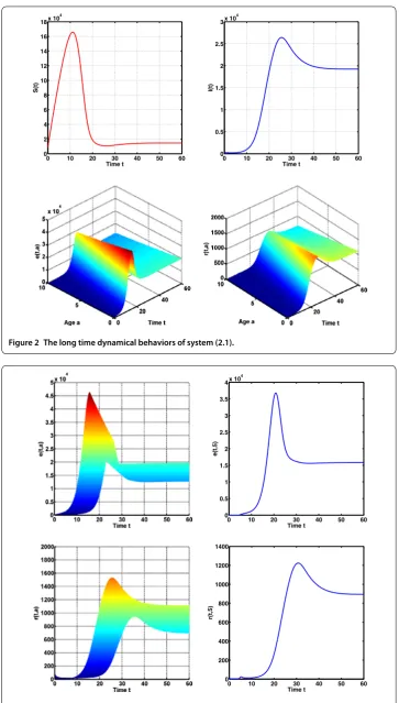
6.1 The long time behaviors of system (2.1)
First, Theorem . asserts that the unique endemic steady stateT∗is globally asymptoti-cally stable. This fact is revealed by Figure . From Figure , one can observe that the lev-els of all compartmental individuals tend to stable values, whereS(t),e(t,a),I(t) andr(t,b) converge to the positive steady statesS∗,e∗(a),I∗andr∗(b). Easily, we can getS∗= .×
andI∗= .×. Obviously, it follows from Figure that the numbers of the exposed
and removed compartments are the distribution functions ofaandb, respectively, partic-ularly,e∗() = .×,e∗() = .×andr∗() = ,,r∗() = . Furthermore,
we show that the distribution ofe(t,a) andr(t,a) for all age and ata= . Figure shows that this is a stationary distribution along all time.
6.2 The age distribution of the latent and removed populations
Figure 2 The long time dynamical behaviors of system (2.1).
Figure 4 Distribution of the latent and removed populations prevalence for all time and att= 40.
Figure 5 Distribution of the latent and removed populations prevalence fort∈[0, 60] and a range of age. Results are obtained fore(t,a) (left) andr(t,b) (right).
6.3 The stationary distribution
7 Conclusion and discussion
In this paper, we proposed and investigated a class of age-structured SEIR epidemic model with immigration. We show that, for all parameter values, the endemic steady state is unique and globally asymptotically stable by using the Lyapunov functional.
All simulation results show that the immigration of individuals leads to the insight that the TB cannot be fully eliminated from the population and will eventually reach a steady endemic level. The age of latent and removed leads to stationary patterns. This implies that TB will exist if either the immigration of population is allowed or there are TB infections in the region. Thus, in order to eradicate the TB, there are two choices: one is to prohibit the immigration of infected individuals, which is difficult to achieve; the other is to clear away the TB in any one region.
Acknowledgements
This work was supported by the National Nature Science Foundation of China under Grant Nos. 11601293 and 11331009, Shanxi Scientific Data Sharing Platform for Animal Diseases (201605D121014), and the science and technology innovation team of Shanxi province (201605D131044-06). We are very grateful to the anonymous referees and editor for their careful reading, valuable comments and helpful suggestions, which have helped to improve the presentation of this work significantly.
Competing interests
The authors declare that they have no competing interests.
Authors’ contributions
The authors contributed equally to this paper. All authors read and approved the final manuscript.
Author details
1Complex Systems Research Center, Shanxi University, Taiyuan, Shan’xi 030006, China.2Key Laboratory of
Eco-environments in Three Gorges Reservoir Region (Ministry of Education), School of Mathematics and Statistics, Southwest University, Chongqing, 400715, China.
Publisher’s Note
Springer Nature remains neutral with regard to jurisdictional claims in published maps and institutional affiliations.
Received: 16 May 2017 Accepted: 27 July 2017 References
1. Daniel, TM, Bates, JH, Downes, KA: History of Tuberculosis: Pathogenesis, Protection, and Control. Am. Soc. Microbiol., Washington (1994)
2. World Health Organization: Global tuberculosis report 2012, Geneva, Switzerland (2012)
3. Bowong, S, Tewa, JJ: Global analysis of a dynamical model for transmission of tuberculosis with a general contact rate. Commun. Nonlinear Sci. Numer. Simul.15(11), 3621-3631 (2010)
4. Ziv, E, Daley, CL, Blower, SM: Early therapy for latent tuberculosis infection. Am. J. Epidemiol.153(4), 381-385 (2001) 5. Feng, Z, Iannelli, M, Milner, F: A two-strain tuberculosis model with age of infection. SIAM J. Appl. Math.62(5),
1634-1656 (2002)
6. Liu, J, Zhang, T: Global stability for a tuberculosis model. Math. Comput. Model.54(1), 836-845 (2011)
7. Yang, Y, Li, J, Zhou, Y: Global stability of two tuberculosis models with treatment and self-cure. Rocky Mt. J. Math.
42(4), 1367-1386 (2012)
8. Martin, SW: Livestock Disease Eradication: Evaluation of the Cooperative State-Federal Bovine Tuberculosis Eradication Program. National Academies Washington (1994)
9. van den Driessche, P, Zou, X: Modeling relapse in infectious diseases. Math. Biosci.207(1), 89-103 (2007)
10. Liu, L, Wang, J, Liu, X: Global stability of an SEIR epidemic model with age-dependent latency and relapse. Nonlinear Anal., Real World Appl.24, 18-35 (2015)
11. Magal, P: Compact attractors for time periodic age-structured population models. Electron. J. Differ. Equ.2001, 65 (2001)
12. Huang, G, Liu, X, Takeuchi, Y: Lyapunov functions and global stability for age-structured HIV infection model. SIAM J. Appl. Math.72(1), 25-38 (2012)
13. McCluskey, CC: Global stability for an SEI epidemiological model with continuous age-structure in the exposed and infectious classes. Math. Biosci. Eng.9(4), 819-841 (2012)
14. Wang, J, Zhang, R, Kuniya, T: Global dynamics for a class of age-infection HIV models with nonlinear infection rate. J. Math. Anal. Appl.432(1), 289-313 (2015)
15. Wang, L, Liu, Z, Zhang, X: Global dynamics for an age-structured epidemic model with media impact and incomplete vaccination. Nonlinear Anal., Real World Appl.32, 136-158 (2016)
16. Webb, GF: Theory of Nonlinear Age-Dependent Population Dynamics. Dekker, New York (1985)
18. Smith, HL, Thieme, HR: Dynamical Systems and Population Persistence. Am. Math. Soc., Providence (2011) 19. McCluskey, CC, van den Driessche, P: Global analysis of two tuberculosis models. J. Dyn. Differ. Equ.16(1), 139-166
(2004)
20. Guo, H, Li, MY: Global stability of the endemic equilibrium of a tuberculosis model with immigration and treatment. Can. Appl. Math. Q.19, 1-18 (2011)
21. McCluskey, CC: Global stability for an SEI model of infectious disease with age structure and immigration of infecteds. Math. Biosci. Eng.13(2), 381-400 (2016)
22. Wang, L, Wang, X: influence of temporary migration on the transmission of infectious diseases in a migrants’ home village. J. Theor. Biol.300, 100-109 (2012)
23. Guo, H, Wu, J: Persistent high incidence of tuberculosis among immigrants in a lowincidence country: impact of immigrants with early or late latency. Math. Biosci. Eng.8(2), 695-709 (2011)
24. Zhang, J, Li, J, Ma, Z: Global dynamics of an seir epidemic model with immigration of different compartments. Acta Math. Sci.26(3), 551-567 (2006)
25. Brauer, F, van den Driessche, P: Models for transmission of disease with immigration of infectives. Math. Biosci.171(2), 143-154 (2001)
26. Grzybowski, S, Enarson, DA: The fate of cases of pulmonary tuberculosis under various treatment programmes. Bull. Int. Union Against Tuberc.53(2), 70-75 (1978)
![Figure 5 Distribution of the latent and removed populations prevalence for tage. Results are obtained for ∈ [0,60] and a range of e(t,a) (left) and r(t,b) (right).](https://thumb-us.123doks.com/thumbv2/123dok_us/961046.1117792/19.595.119.479.81.385/figure-distribution-latent-removed-populations-prevalence-results-obtained.webp)