Routing in delay tolerant networks with periodic connections

(1)

R E S E A R C H

Open Access

Routing in delay tolerant networks with

periodic connections

Cem Mergenci

*

and Ibrahim Korpeoglu

Abstract

In delay tolerant networks (DTNs), the network may not be fully connected at any instant of time, but connections occurring between nodes at different times make the network connected through the entire time continuum. In such a case, traditional routing methods fail to operate because there are no contemporaneous end-to-end paths between sources and destinations. This study examines the routing in DTNs where connections arise in a periodic nature. We analyze various levels of periodicity in order to meet the requirements of different network models. We propose different routing algorithms for different kinds of periodic connections. Our proposed routing methods guarantee the earliest delivery time and minimum hop-count, simultaneously. We evaluate our routing schemes via extensive simulation experiments and compare them to some other popular routing approaches proposed for DTNs. Our evaluations show the feasibility and effectiveness of our schemes as viable routing methods for delay tolerant networks.

Keywords: Delay tolerant networks, Routing, Periodic connections

1 Introduction

In delay tolerant networks (DTNs) [1] an end-to-end path between a source and destination is not guaranteed to exist at any time instant. Connections between nodes at different times provide an end-to-end path in the future, therefore, connecting the network throughout the entire time continuum. This condition causes DTNs to suffer from large delays. Long disconnection times and parti-tions in the network are also typical problems, which make communication in DTNs a challenging task.

Not all network applications are suitable to run over DTNs. Applications requiring a continuous flow of data, such as multimedia streaming, or requiring a connec-tion to be present, such as secure shell (SSH) or instant messaging (IM), are not good candidates to run in a high-delay, disconnected environment. On the other hand, some applications can tolerate large delays and therefore can still work as expected in a high-delay environment. Email, Domain Name System (DNS), BitTorrent [2] are good examples of delay tolerant applications.

*Correspondence: mergenci@cs.bilkent.edu.tr

Department of Computer Engineering, Bilkent University, Ankara, Turkey

As well as the existing applications, very different appli-cation types have emerged with the DTN concept, such as contextual applications using locally available data. For example, a social networking application running on the mobile handsets of conference participants in different locations, can collect the profiles of attendees and sug-gest which people have similar interests. Vehicular ad-hoc networks (VANETs), military ad-hoc networks, wireless sensor networks (WSNs), satellite, and free-space com-munication [3] are other fields in which delay tolerant networking concepts can be applied.

The main problem with DTNs is that existing network-ing protocols in use today, such as the ubiquitous TCP/IP protocols, assume the availability of an end-to-end path and acceptable round-trip times in communication. These assumptions make the methods unsuitable for a DTN environment [4]. Even mobile ad-hoc network (MANET) routing protocols such as AODV [5] and OLSR [6] are not designed to work in a delay tolerant environment. As a result, different sets of networking protocols have been devised for DTNs to meet various requirements.

In this paper, we examine the routing issue in DTNs with periodic connections. We begin the paper with an analysis

(2)

of a simple connection model, in which contacts occur at a given future time with no periodicity. We propose an algo-rithm based on Dijkstra’s shortest path algoalgo-rithm, with customizations to meet the requirements of this simple connection model. This algorithm guarantees the earli-est delivery (ED), and therefore, is optimal in terms of time. Then, we extend the connection model to incor-porate periodic connections, which is the main focus of this paper. In this model, contacts occur first at a given time and repeats at certain intervals. We revise our rout-ing algorithm to compute future contact times from the new connection model by taking periodicity into account. This connection model assumes contact durations to be insignificant such that a connection becomes available and unavailable instantly, though allowing enough time for packet exchanges.

Assuming that very short contact durations may not be applicable to all cases, we extend our connection model to include significant connection durations. The new con-nection model has separate concon-nection and disconcon-nection states lasting different durations. Again, connections and disconnections occur periodically in an alternating fash-ion. We provide the most general version of our ED routing algorithm using this connection model. It com-putes future contact times accordingly and exploits the connection periods.

Earliest delivery routing is optimal in time, but not in hop count. The greedy approach taken by the algorithm (similar to the greedy approach taken by Dijkstra’s short-est path algorithm) produces routes that are suboptimal in hop count. We address this problem with our min-hop earliest delivery routing (MHED) algorithm, which finds paths that guarantee the earliest delivery and are also minimal in hop count. We consider two types of MHED, one based on a Dijkstra-like approach and one based on a breadth-first search (BFS) approach. The running time analysis reveals that the BFS-based and Dijkstra-based MHEDs both run asymptotically equally fast, but we conclude that the BFS-based MHED is more practical. We also present a strictly min-hop (MH) routing scheme as a complement to MHED routing. Min-hop routing is not optimal in delivery time; however, it not only routes through the shortest path in terms of hop count, but also chooses the earliest delivery path among minimum hop paths.

The rest of the paper is organized as follows: Section 2 gives some background to and related work in DTN routing, comparing and contrasting those works with our study. Section 3 defines the routing problem for DTNs with periodic connections and proposes differ-ent routing solutions for differdiffer-ent connection models. Section 4 explains our experiments and evaluates the results. Section 5 concludes the paper, and gives exten-sions and future research directions on the topic.

2 Related work

In [7], the authors formulate a DTN routing problem given the connectivity patterns of nodes, then present a compre-hensive framework for evaluating and classifying different routing algorithms. A thorough examination of routing algorithms by strategies employed such as forwarding, replication, and coding [8] is given in [9]. The study offers a guideline for choosing a proper routing method for DTNs with different characteristics. Woungang et al. [10] presents a broader view of routing in opportunistic networks including DTNs, MANETs, and VANETs.

In [11], the authors apply the epidemic algorithm con-cept of [12] to partially connected ad-hoc networks. Nodes buffer messages they receive even if they do not know a route to the destination. When two nodes come into contact, they exchange messages. In this way, a mes-sage is delivered to every contacting node and finally delivered to its destination.

Similar to epidemic routing, PROPHET [13] introduces probabilistic routing decisions. Every node maintains a delivery predictability for each node it encounters. Nodes that meet frequently have higher delivery predictability, and this aspect decreases if nodes do not encounter each other for a while. Epidemic forwarding of packets occurs only when the delivery predictability of a neighbor is higher than that of the node itself for a destination.

Single-copy routing schemes are presented by [14]. These strategies depend on the fact that every local pro-gression will lead a packet to its destination. In the most basic strategy, direct transmission, the source node for-wards the packet only if it encounters the destination. In utility-based routing, nodes forward a packet only if a neighbor has a higher utility value to the destination.

Another single-copy technique is proposed by [15]. Using only average inter-contact time estimates between nodes, a 2-hop relay strategy is extended to a recursive multi-hop relay strategy.

Spray and Wait routing [16] aims to compromise between epidemic routing and single-copy routing by lim-iting the number of copies a packet can have. It reduces the number of transmissions with respect to epidemic routing and achieves a better delivery ratio than single-copy schemes.

(3)

to live, lower hop count, and smaller size. Buffering effi-ciency is examined in detail in [21]. Based on a Markov chain model, the authors analyze the effect of bundle sizes to storage requirements and delivery success.

In [22], the authors discuss routing in networks with predictable mobility. Nodes follow a certain determin-istic trajectory that is defined as a function of time. Given any time instant, a network graph can be con-structed from the node locations. A space-time graph is the combination of different network graphs at different time instants in a single large graph, on which routing is performed.

The authors of [23] focus on scalability issues in routing for DTNs. Under the same mobility model defined by [22], they propose DTN Hierarchical Routing (DHR), which applies hierarchical routing to multiple levels of a multi-level clustered network. Another study [24] examines thoptimality issue for probabilistic forwarding protocols. Authors define a 1-hop delivery probability metric and extend it to K-hops. The forwarding rule defined using the metric is formulated inside an optimal stopping rule problem to find optimal routes.

Liu and Wu [25] focus on DTN routing under cyclic mobility patterns. The study assumes that the probability of contact between two nodes is higher if they have been in contact in previous cycles. A probabilistic time-space graph model is converted to an equivalent timeless prob-abilistic state-space graph, on which a Markov decision process is applied to calculate expected minimum delay (EMD) routing.

Various studies define routing metrics based on one or more network properties. Dvir and Vasilakos [26] present a backpressure-based routing algorithm. Lindgren et al. [13] use frequency of contacts, and [27] use elapsed time since last contact. Daly and Haahr [28] and Hui et al. [29] use similar techniques, defining betweenness, centrality, and social similarity of nodes as routing metrics. Bulut et al. [30] propose Conditional Shortest Path Routing (CSPR) based on a routing metric (conditional intermeet-ing time) that defines the time two nodes meet over an intermediate node. Ayub et al. [31] combine statistics such as recent encounters and transmit, drop, and receive counts to calculate a per contact quality point, which determines forwarding and buffering decisions. Routing metrics of cognitive radio networks is surveyed in [32]. Presented framework can be applied to DTN routing metrics.

Practical concerns about DTN routing are examined in [33]. The presented protocol depends on an estimate of how long a message waits on a host until transmission to the next hop. The estimate is calculated from contact his-tory, therefore does not use global contact information. Forwarding is performed when a neighbor is estimated to be closer to the destination than the current node.

According to the classification in [7], our study uses only contact information. We do not utilize queueing or traf-fic demand for routing decisions; therefore, our approach is a partial knowledge routing method. As noted earlier, we use routing algorithms based on Dijkstra’s algorithm. Using contact information eliminates the need for proba-bilistic routing decisions.

We propose a single-copy routing scheme, as opposed to multi-copy schemes such as epidemic routing or spray-and-wait. However, our algorithms ED and MHED are similar to epidemic routing in terms of delivery time; both are optimal strategies guaranteeing the earliest delivery.

We focus on how connections are established, regard-less of the reason behind it, whether it is mobility, avail-ability, scheduling, or interference. Therefore, our study is different than [22], [23], and [25], as our approach enables us to devise exact routing algorithms that are general enough to be tailored to various contexts in delay tolerant networking.

To the best of our knowledge, we are the first to address minimum hop and earliest delivery objectives together in a routing algorithm in the context of DTNs.

3 Our proposed DTN routing protocols

In our delay tolerant network model, we assume that connection opportunities arise periodically between two nodes. This assumption is realistic due to the fact that interactions between entities and people are periodic in nature. As academic professionals, we see our colleagues every morning, friends from other departments at lunch, and our family in the evening. Similarly, students interact in class and during breaks. Vehicles in public transporta-tion arrive at statransporta-tions periodically [34]; sensors periodi-cally transmit data to base stations and so on.

We identify three cases of connection models of increas-ing complexity. In the first model, contacts occur only once in the future. The second model introduces periodic connections with negligible connection durations. Finally, the third model considers both connection and discon-nection durations separately for periodic condiscon-nections.

(4)

3.1 Routing for DTNs with scheduled one-time connections

We begin with a simple connection model, in which con-nections occur only once according to a predetermined schedule. We can calculate perfect shortest routes given source, destination, packet generation/arrival time, and connection establishment time between nodes. We fur-ther simplify the model by neglecting contact durations, which we consider in later versions. An established con-nection is assumed to be lost as soon as all the necessary packets have been exchanged between two nodes. Start-ing with such a simple model facilitates developStart-ing the algorithms for the more complex periodic connections cases.

3.1.1 Basic model

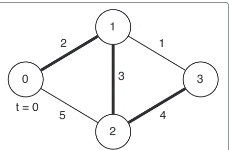
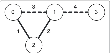
We let edge weights,w(u,v), represent the contact times between nodes in a DTN environment. Figure 1 shows an example network. The link between Nodes 0 and 1 will be available att=2, the link between Nodes 0 and 2 will be available att=5, and so on.

In such a scenario, the shortest path is redefined to be the shortest path in time with non-decreasing edge weights because a decreasing edge weight from one link to another would mean a missed contact opportunity. This method implies that if a non-decreasing weight path does not exist for a vertex, that vertex is not reachable from the source.

Figure 2 shows the routing tree of Node 0 at t = 0. Node 1 is reachable att=2. Although Node 2 is directly reachable att=5, there exists a shorter path where pack-ets destined to Node 2 can be delivered at t = 3 over Node 1. The shortest path to Node 3 is over Node 2 at t = 4. The link between Nodes 1 and 3, available only att=1, cannot be utilized since packets arrive at Node 1 att=2 at the earliest.

The shortest distancet[u] to a vertexufrom the source is also redefined to be the time a packet generated att=0

Fig. 1Example network with scheduled one-time connections

Fig. 2Routing tree of Node 0 att=0 in the network in Fig. 1

is delivered. In the network given in Fig. 1, the shortest distances to Nodes 1, 2, and 3 from Node 0 are 2, 3, and 4, respectively.

The original vertex relaxation algorithm refined to work under these conditions is given in Algorithm 1. The con-dition in the if-statement checks whether the edge is in a non-decreasing order in the path. Edge weights are not accumulated as in the original version because they are absolute contact times.

Algorithm 1 Vertex relaxation for scheduled one-time connections

REL AX(u,v,w)

1: ifw(u,v)≥t[u] andt[v]>w(u,v)then 2: t[v]←w(u,v)

3: π[v]←u 4: end if

3.1.2 Routing at t>0

So far we have discussed how to compute a routing tree at t = 0. Algorithm 2 is a simple modification of the INITIALIZE-SINGLE-SOURCE(G,s) in Dijkstra’s algorithm, to enable the shortest route computation at an arbitrary timet.

Algorithm 2 Initialization of Dijkstra’s algorithm with timet

INITIALIZE-SINGLE-SOURCE(G,s,t) 1: for allv∈V[G]do

(5)

The initial distance to the source is set to givent. The source node remains the first node to be extracted from the min-heap, sincetis smaller than the initial distances of all other nodes,∞. The relaxation method in Algorithm 1 considers only edges that have contact times now or in the future; therefore, the non-decreasing edge weight path property is still maintained.

The signature of the main routing Dijkstra procedure should be updated to DIJKSTRA(G,w,s,t) to accept the timetat which the routing tree will be computed as.

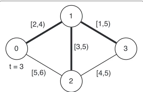
Figure 3 shows the routing tree for Node 0 att=3. Only Node 2 is reachable att=5, as the contact opportunities of others are lost either att=3 ort=5.

3.2 Routing for DTNs with scheduled periodic connections

In this section, we extend our network model to uti-lize periodic connections that occur according to a pre-defined schedule. We first examine the case where contact durations are insignificant and then consider periodic connections with significant contact times.

3.2.1 Insignificant contact durations

We assign each edge (u,v) a period T(u,v) after which connection is reestablished. In this model, no vertex is unreachable (as long as the space-time graph representing DTN is connected), because a connection will be available after at mostT(u,v) time. As stated earlier, we assume that the graph representing possible connections among nodes is a connected graph. All nodes have connection opportunities to all other nodes.

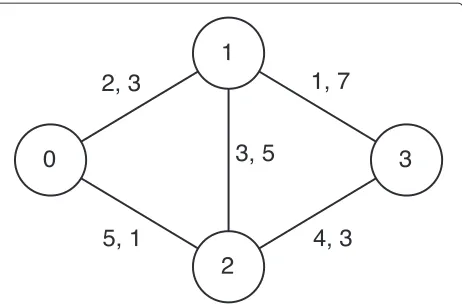
Figure 4 shows an example network with periodic con-nections. Each link is tagged with a pair (w,T), where w represents the initial wait time of a link, after which connections begin to occur with periodT. For example, the link between Nodes 0 and 1 becomes available at t = 2 and then comes up again at every 3 units of time,

Fig. 3Routing tree of Node 0 att=3 in the network in Fig. 1

Fig. 4Example network with initial wait times and connection periods

t = {5, 8, 11, 14,. . .}. The function in Eq. 1 gives thekth connection time for a link(u,v):

f(k,u,v)=w+k·T(u,v) (1)

The routing tree for Node 0 at t = 0 is identical to the one depicted in Fig. 2 because exact schedules in the scheduled one-time connection case correspond to initial wait times in the periodic connection case. However, the routing tree att = 3, shown in Fig. 5, is different than that in Fig. 3. The time signatures on the edges denote when a link becomes available at the closest point in time after one of its nodes receives a packet from Node 0 at timet. All the nodes are reachable in this case because connections arise periodically.

Algorithm 3 extends the Relax(u,v,w) given in Algorithm 1 with another parameter for connection peri-ods. The statement inside the first condition calculates the first connection time after t = t[u] using T(u,v). The first condition in the if-statement of Algorithm 1 is no longer needed since we ensure the weights are non-decreasing with this initial calculation.

(6)

Algorithm 3 Vertex relaxing for insignificant contact durations

REL AX(u,v,w,T) 1: ifw(u,v) <t[u]then

2: w(u,v)←w(u,v)+T(u,v)·

t[u]−w(u,v) T(u,v)

3: end if

4: ift[v]>w(u,v)then 5: t[v]←w(u,v) 6: π[v]←u 7: end if

Throughout the execution of the algorithm, whenever w(u,v)is assigned, it is assigned the next connection time of the corresponding link.

3.2.2 Significant contact durations

So far we have assumed that connections remain avail-able for a negligible amount of time. This assumption is not very realistic, as connection times are compara-ble to disconnection times. To alleviate this procompara-blem, we define TON(u,v) and TOFF(u,v) to be connection and disconnection durations between nodes u and v, respectively. In this case, the original period definition becomesT(u,v) = TON(u,v)+TOFF(u,v). Connection and disconnection phases alternate after the initial wait time.

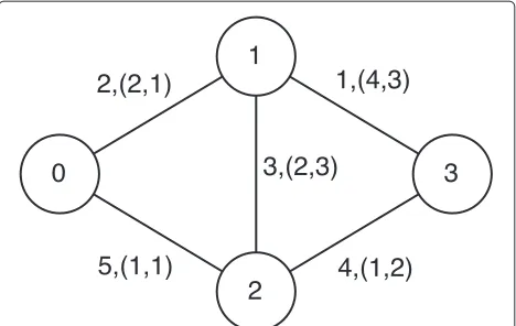
Figure 6 shows a network with significant contact dura-tions. Links are labeled with triple (w, (TON, TOFF)). A link first goes up at the end of its initial wait time, w. The connection lasts forTON time, after which a discon-nection occurs forTOFF time.ON andOFFstates follow each other after that point. For instance, the link between Nodes 0 and 1 becomes available at t = 2, disconnec-tion occurs at t = 4, and the next connection period begins at t = 5. The functions in Eqs. 2 and 3 give

Fig. 6Example network with initial wait times, connection, and disconnection periods

the beginning of the kth _{connection and disconnection} periods, respectively, for a link(u,v):

fON(k,u,v) = w+k·T(u,v) (2) fOFF(k,u,v) = w+TON(u,v)+k·T(u,v) (3)

The routing tree for Node 0 att = 3 is illustrated in Fig. 7. For each link in the figure, the next time interval just after or including the current time during which the link is on, is given as the link label. When a nodeureceives a packet att[u], it can forward it to nodevatt[v]= t[u] if they are connected at that time (i.e., the link is on at that time). Otherwise, nodeushould wait until the begin-ning of the next connection to forward the packet, as in previous cases. In the example in Fig. 7, every destination receives the packet att= 3, as all the links are on at that time.

Algorithm 4 defines the relaxation method for the sig-nificant contact durations model. w(u,v) keeps track of the beginning time of the last ON period.

Algorithm 4Vertex relaxing with arbitrary initial wait times REL AX(u,v,w,TON,TOFF)

1: ifw(u,v)+T(u,v)≤t[u]then

2: w(u,v)←w(u,v)+T(u,v)·t[u_T]−₍_uw_,(_vu₎,v)

3: end if

4: ifw(u,v)≤t[u]then Initial wait time has passed

5: ift[v]>t[u] andt[u]<w(u,v)+TON(u,v)then

6: t[v]←t[u] (u,v)is up att=t[u]

7: π[v]←u

8: else ift[v]>w(u,v)+T(u,v)then 9: t[v]←w(u,v)+T(u,v)

10: π[v]←u

11: end if

12: else ift[v]>w(u,v)then 13: t[v]←w(u,v)

14: π[v]←u

(7)

Fig. 7Routing tree for Node 0 att=3 in the network in Fig. 6

3.3 Min-hop earliest delivery routing

So far, we have discussed routing to achieve earliest delivery-routes that are shortest in time. In this section, we define the shortcomings of earliest delivery routing and introduce min-hop earliest delivery routing.

3.3.1 Motivation for Min-hop earliest delivery routing Suppose we have the network in Fig. 8 with scheduled one-time connections.

The earliest delivery algorithm run in Node 0 would find the route to Node 3 as [0, 2, 1, 3], witht = 4 being the delivery time. However, there exists a shorter route if we consider hop-count as a secondary metric: route [0, 1, 3] is shortest in delivery time (t =4) and hop count (h=3 vsh=2).

The previous algorithms fail to detect such a route because they make greedy choices based only on deliv-ery time. The route to Node 1 from Node 0 travels over Node 2, reaching Node 1 earliest. Once we set Node 2 as the parent of Node 1, all routes descending from Node 1 in the routing tree travel over Node 2 independent of their time. However, we can choose any other route to Node 1 for routing packets destined to nodes that are chil-dren of Node 1 in the original routing tree, as long as the

Fig. 8Example network where ED and MHED differ

non-decreasing edge weight path property is satisfied end to end. In this case, path [0, 1] witht = 3 satisfies the non-decreasing edge weight path property for path [1, 3] witht=4; therefore, we can choose path [0, 1, 3] to route packets from Node 0 to Node 3. Since we are trying to find min-hop routes, the paths we choose should be shorter in terms of hop count.

Reducing hop count means reducing the number of transmissions in a practical setting. In environments where energy is constrained, such as in a network of mobile handsets, the number of transmissions becomes an important factor in communications. Wireless sensor networks is another domain where energy conservation is important. In such cases, having fewer transmissions prolongs network lifetime.

3.3.2 Routing tree

In the routing tree concept, every node has a parent node through which it receives packets. In min-hop earli-est delivery routing, the routing tree concept is different; every edge through which packets are routed has a par-ent edge. This method causes a node to appear in differpar-ent branches of the routing tree; however, an edge can appear only on a single branch.

Figure 9 shows the routing tree of min-hop earliest delivery routing for the network in Fig. 8. There are two branches in the routing tree, as shown in Fig. 9. Node 1 appears on the top branch as an intermediate node en route to Node 3 and as a terminal node on the bottom branch. Figure 10 presents an alternative view, showing the routing tree inside the network graph.

3.3.3 MHED data structures

The solution to MHED routing comes from the observa-tion that we should utilize paths that are shorter than the earliest delivery path in hop count. Among those paths having the same hop count, we should still choose the path providing the earliest delivery so that the resulting path is the shortest. We are not interested in paths that are longer than the earliest delivery path in hop count because the earliest delivery path is always shorter.

(8)

Fig. 10Min-hop earliest delivery routing tree for network of Fig. 8, an alternative view

Another important observation is that any-number-of-hop paths to a vertex may become the shortest path for a neighbor vertex. This observation is illustrated in Fig. 11.

Assuming Node 0 is the source, the earliest delivery path to Node 4 is [0, 1, 2, 4], with h = 3 (hops) and t = 3. The ED algorithm would route all the packets to Nodes 5 and 6 through this path over Node 4; however, there are shorter alternatives. The shortest path to Node 5 is [0, 3, 4, 5] (h=3,t=5), and to Node 6 is [0, 4, 6] (h=2,t=7). The shortest paths to both Nodes 5 and 6 is still through Node 4, but the route uses different paths with different numbers of hops until Node 4. In this example, all possible number-of-hop paths (1-hop, 2-hop, 3-hop) to Node 4 are utilized as a shortest path to a node.

As a result, our solution should keep track ofn-hop ear-liest delivery routes to all nodes, wheren≤hop count of the earliest delivery path.

The initialization of the MHED algorithm’s data struc-tures is given in Algorithm 5. hop[v] is the hop count of the earliest delivery path to a vertex. t[v,n] and π[v,n], respectively, hold the earliest delivery time of and parent vertex for an n-hop path to vertexv. There-fore, t[v,hop[v] ] and π[v,hop[v] ] correspond to t[v] and π[v], respectively, in the earlier initialization pro-cedure, INITIALIZE-SINGLE-SOURCE(G,s,t), defined in Algorithm 2. Lastly, the earliest delivery time of source node at 0 hops is set tot.

Fig. 11Example network with many MHED routes

3.3.4 MHED algorithm

In the main algorithm, we should traverse the graph and fill the data structures at the nodes with the correct values and therefore obtain the routing tree. The objective is to find then-hop earliest delivery paths to each vertex. We already know that previous algorithms based on Dijkstra’s algorithm achieve the earliest delivery. Now, we also keep track of hop counts together with earliest delivery times. We modify the min-heap structure to keep hop-vertices, a two-tuple(u,n), whereuis the vertex andnis the hop count. Comparison between two hop-vertices is done in the order of hop and delivery time to the vertex atnhops. Equation 4 gives the formal definition of theminfunction used by the min-heap.

The min function implies that all n-hop hop-vertices will be extracted from the heap before an (n+1)-hop hop-vertex is extracted.

(9)

Algorithm 6 MHED algorithm based on Dijkstra’s

The relax function in Algorithm 7 takes hop countn, after which edge(u,v) is reached. The first condition in the if-statement checks whether this edge satisfies the non-decreasing edge weight path property after traveling then-hop path to vertexu. The second condition checks whether this edge constitutes a shorter path than up to n-hop paths to vertexv. Because of the way hop-vertices are extracted from the min-heap,hop[v] is never greater than n + 1 and converges to the path length of the earliest delivery path throughout the execution. If both of these conditions hold, it means edge (u,v) forms an (n+1)-hop path to v. If hop[v]< n+ 1, we need to insert a new hop-vertex in the heap; if it is not, the hop-vertex is already in the heap and we need to per-form a DECREASE-KEYoperation. DECREASE-KEY, which was implicit in previous versions, is explicitly written for clarity.

Note that inserted hop-vertices can have a hop count of n + 1. By the definition of the min function over hop-vertices, alln-hop hop-vertices are extracted before (n+1)-hop ones. It can be concluded that only n-hop and (n+1)-hop hop-vertices can occur in the heap at the same time. Therefore, the hop difference between the minimum and maximum hop hop-vertex is at most 1.

This property is the same as the property of a BFS queue in operation; therefore, we can substitute min-heap with a

first-in, first-out (FIFO) queue. Algorithm 8 presents the MHED algorithm based on a BFS. The only difference from the Dijkstra-based version is the use of queue oper-ations instead of min-heap operoper-ations.

Algorithm 8MHED algorithm based on a BFS MHED(G,w,s,t)

Vertex relaxing requires some modifications. Since we are not using a min-heap, we can omit the DECREASE-KEY operation, which is implicitly satisfied by the ordering in the queue, and use ENQUEUE instead of INSERT. Vertex relaxing for a BFS-based MHED is given in Algorithm 9.

For the sake of brevity, in Algorithm 9, we omit the insignificant contact durations connection model and give the MHED relaxation procedure for significant contact durations with arbitrary initial wait times. The MHED relaxation routine corresponds to the ED relaxation rou-tine defined in Algorithm 4. The main difference from the previous versions is the use of a temporary variablew instead of the actualw(u,v). We do this because a vertex is enqueued multiple times (once for each hop), there-fore its edges are traversed multiple times. If we were to assign connection times to w(u,v), the values might not be correct for subsequent times. By using the tempo-raryw, the next contact time is calculated from the initial w(u,v)every time, regardless of how many times a vertex is dequeued.

(10)

Algorithm 9Vertex relaxing for a BFS-based MHED

3.3.5 Running time analysis of MHED

We begin the running time analysis of the BFS-based MHED, by inspecting the number of iterations of the while-loop in Line 4 of Algorithm 8. The while-loop runs until there are no hop-vertices left in the queue; therefore, the iteration count is equal to the number of enqueue and dequeue operations. As discussed earlier, there can be at most|Adj[v]|number ofn-hop paths to a vertexv, if every neighbor provides a path with a different number of hops from the source. Considering the whole graph, all vertices cannot have incoming paths from all of their neighbors since some of the edges will be used for outgoing paths. More specifically, the edges of a vertex through which a new vertex is discovered cannot constitute an n-hop path to that vertex. Aggregating the number of n-hop paths up to all vertices gives the number of edges, |E|. As a result, there are at most|E|number of hop-vertices, enqueue, and dequeue operations.

2|E|2

|V| . The relaxation method runs in constant time, since

every statement, including the enqueue operation on the FIFO queue, takes constant time.

The initialization procedure takes O(V2) time; therefore, the running time of the BFS-based MHED algorithm is O

V2+ E_V2

, which is always between

O(V2)andO(V3)for an arbitrary network.

The Dijkstra-based MHED algorithm uses insert and extract-min operations on a min-heap instead of enqueue and dequeue operations on a FIFO queue. The implica-tion is that the min-heap is the same size as the BFS queue, which isO(V)in size. There are also decrease-key operations inside the relax method.

Using a binary heap, insert and extract-min opera-tions takeO(ElgV)time on the aggregate. Decrease-key operations may occur in every iteration of the for-loop except when insert is called, therefore making the aggre-gate run timeO and for-loop iterations, overall running time becomes

O

Using a Fibonacci heap, extract-min operations take OElgV amortized time and the running time of the

decrease-key operations decreases to O

E2

V

amortized time. Taking the initialization procedure and for-loop iter-ations into account, the amortized running time of the Dijkstra-based MHED algorithm using a Fibonacci heap is O

Although the running times of the BFS-based and the Dijkstra-based Fibonacci heap solutions are the same, the former has a worst case and the latter has an amortized running time. When the simplicity of a FIFO queue is also considered over the complexity of a Fibonacci heap, we conclude that the BFS-based approach is preferable to the Dijkstra-based approach.

3.4 Min-hop routing

Min-hop earliest delivery routing achieves optimal deliv-ery time while using the minimum number of hops possi-ble. A natural successor is MH routing, which is optimal in hop count while achieving the earliest delivery time pos-sible. It could be called earliest delivery min-hop (EDMH) routing, but we simply call it min-hop routing because it is trivial to achieve earliest delivery while finding min-hop routes.

Min-hop routes are already computed within the MHED procedure. Since the algorithm finds all n-hop paths to a vertex with corresponding delivery times, the smallestnsuch thatt[v,n]= ∞for a vertexvgives the MH value.

(11)

route to the reached vertex. Details are omitted for brevity.

The MH procedure runs in linear time,O(E+V), the same as a BFS.

4 Simulation experiments and evaluation

In this section, we present the experiment results of the proposed DTN routing algorithms and evaluate the find-ings. We first define the simulation environment and the properties and parameters of the simulations, then discuss the results and their implications.

4.1 Simulation properties

We performed simulations to find the properties of our routing algorithms for different parameter values. We measured transmission count, average path length to destination, delivery time, and routing tree stability statistics. Implementation was done on a Java platform using a custom graph and routing code. Simulations were run on a Linux machine with a quad-core AMD 64-bit processor and 4 GB memory, though the min-imum requirements for the implementation are much lower.

We performed a simulation as follows: First, a ran-dom graph was generated with a given node count, connection model, and network density with a unit of d = ₍_|_V_|₍2_||_VE_|−| ₁₎₎. Then, measures were taken over a time interval of 16 h of simulation time, separately for each node as the source. Similarly, the remaining node became the destination for each source node. The results at each step were averaged. The overall procedure was repeated 30 times to ensure enough randomness and samples.

We produced random graphs given the vertex count and graph density. Since DTNs are connected graphs, we needed to ensure our random graph was connected. To achieve this, we had two sets of vertices: connected and disconnected. Until the graph became connected, we chose one random node from the set of connected vertices and one from the set of disconnected vertices and then connected them. When all of the vertices were connected, we had a connected graph with |V| − 1 number of edges. Then, we added edges by randomly choosing two vertices until the density constraint was satisfied. Note that the produced graph cannot have a lower density than the density of a minimally connected graph,_|_V2_|d.

For some of the experiments, we considered two sce-narios with different connection models. Scenario 1 sim-ulated a DTN on a university campus. Nodes repre-sented college students attending 50-min lectures and having 10-min breaks. We assumed that connections occured mainly during break times, though we took into account slightly shorter and longer connections and

disconnections. Therefore,TON ranged between 5 and 20 min and TOFF ranged between 15 and 60 min. The key property of this scenario is the fact that connections take less time than disconnections.

Scenario 2 was a more homogenous environment, where connection and disconnection periods were the same. It simulated connection properties of a public trans-portation network. Nodes represented vehicles (bus, sub-way, etc.) and passengers. Connections occurred either in stations or during travel. We assumed that the waiting time for a vehicle and travel time were similar; therefore, TON andTOFFvalues had a range between 10 and 30 min. For both scenarios, we used an initial wait time between the minimum and maximum of the connection or dis-connection times. For Scenario 1, it was 5 to 60 min; for Scenario 2, it was 10 to 30 min. Actual values for each con-nection were drawn from a uniform distribution between determined intervals.

In the experiment results, ED refers to the earliest deliv-ery algorithm based on original Dijkstra’s algorithm using the vertex relaxing procedure in Algorithm 4. MHED refers to the min-hop earliest delivery algorithm based on a BFS, presented in Algorithm 8 using the vertex relax-ing procedure in Algorithm 10. Min-hop routes were computed using MHED data structures, as defined in Section 3.4.

4.2 Results and evaluation

This section presents the evaluation of our experiment results. We analyzed our algorithms in terms of transmis-sion count, path length, delivery time, and routing tree stability.

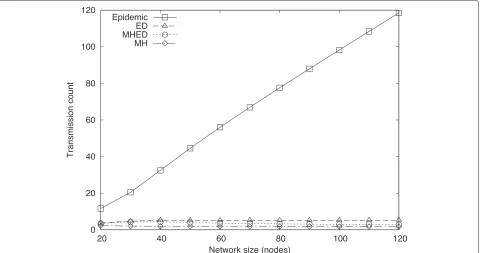
4.2.1 Transmission count

Epidemic routing was one of the earliest and remains one of the most popular routing algorithms for DTNs. The source node forwards its packet to every node it encounters and those nodes forward the packet to their encountered nodes in turn, eventually delivering the packet to the destination at some time in the future. This scheme is aptly called epidemic flooding. Although ED and MHED algorithms are single-copy routing strategies utilizing contact information, they are comparable to epi-demic routing in terms of delivery time. All three methods guarantee earliest delivery.

Figure 12 shows the average transmission count to deliver a single packet to a destination for epidemic, ED, MHED, and MH routing in a network with a density of 0.2d. The figure shows the results for Scenario 1, and trend for Scenario 2 is very similar.

(12)

Algorithm 10Vertex relaxing of MHED with significant contact durations REL AX(u,v,w,TON,TOFF)

1: τ ←w(u,v) 2: relax←false

3: ifw+TON(u,v)≤t[u,n]then

4: w←w+T(u,v)·

t[u,n]−w T(u,v)

5: end if

6: ifw≤t[u,n]then Initial wait time has passed

7: ift[v,hop[v] ]>t[u,n] andt[u,n]<w+TON(u,v)then

8: t[v,n+1]←t[u,n] (u,v)is up att=t[u,n]

9: π[v,n+1]←u 10: relax←true

11: else ift[v,hop[v] ]>w+T(u,v)then 12: t[v,n+1]←w+T(u,v)

13: π[v,n+1]←u 14: relax←true 15: end if

16: else ift[v]>wthen 17: t[v,n+1]←w 18: π[v,n+1]←u 19: relax←true 20: end if

21: ifrelaxandhop[v]<n+1then 22: hop[v]←n+1

23: ENQUEUE(Q, (v, n+1)) 24: end if

(13)

better comparison, we count only the number of trans-missions until the packet reaches the destination. The transmission count of epidemic routing increases linearly with the number of nodes in the network. This method delivers the packet to 90 % of the network with a node count of as low as 50. For higher node counts, the deliv-ery ratio increases to 97 % on the average. With ED and MHED, routing earliest delivery is achieved with very few transmissions, MHED performing better than ED. The MH method achieves the lowest transmission counts of all the methods; however, it is not optimal in time, therefore it delivers packets later than the other methods. This is evident in the delivery time results in Section 4.2.3.

We conclude that ED and MHED successfully uses contact information to deliver packets with much fewer transmissions compared to epidemic routing.

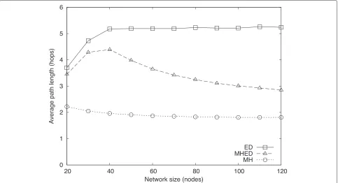
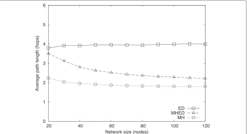
4.2.2 Path length

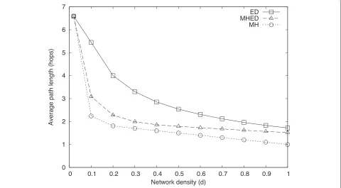
In this experiment, we measure average path lengths (hop counts) to a destination for different network sizes (number of nodes). Note that since all the methods are single-copy routing schemes, average path length corre-sponds to average transmission count.

Figures 13 and 14 show results in a network with den-sity of 0.2d. Intuitively, because the network grows, one expects average path length to increase as the num-ber of nodes in the network increases. Inspecting MH

results, however, shows that our hypothesis does not hold. Even though the number of nodes increases, the average breadth of the network stays almost the same because we construct the network by connecting disconnected ver-tices randomly to connected ones. Such a procedure does not produce wider graphs, but graphs with similar aver-age path lengths. Since the averaver-age path length does not change with network size, we can conclude that the num-ber of alternative routes between two nodes increases as the network size increases.

Increasing the number of alternative routes becomes a disadvantage for ED routing. The greedy choices it can make among more alternatives result in longer paths on the average. On the other hand, MHED routing uses alternative routes to its advantage and decreases average path length. The MH results show distance to destination in the minimum number of hops. This method is suboptimal in delivery time, however, min-imizing hop count first, therefore the values are the same for both scenarios. The MH approach repre-sents a lower bound in path length for any routing method. As the number of nodes increases, the path length of MHED routes moves closer to the lower bound.

The MHED results for Scenario 1 display a maximum at smaller network sizes. This is a practical maximum, occurring because there are fewer alternative paths in smaller networks and those alternatives do not constitute

(14)

Fig. 14Average path length to destination in a network withdensity=0.2dunder Scenario 2

an earliest delivery path shorter in hop count. Increasing the number of alternative paths increases the probabil-ity of achieving shorter earliest delivery paths; after some point, MHED routes become shorter.

Comparing different scenarios, the average difference between ED and MHED routes is greater in Scenario 1 than in Scenario 2. As every other parameter is the same for the two scenarios in this experiment, the explanation of the difference is found in the connection profiles. Dis-connection times in Scenario 1 are greater than those in Scenario 2, on the average. Higher disconnection times make next-connection opportunities later, therefore giv-ing MHED a greater time interval to find routes in fewer hops.

Another difference between the scenarios is the path length, regardless of the algorithm. Paths in Scenario 2 are shorter than those in Scenario 1. The explanation for this result is very similar to the previous one. Due to longer disconnection times in Scenario 1, ED and MHED search for shorter paths in time by increasing the hop count. Since disconnection times are already shorter for Scenario 2, the algorithms are more likely to find earlier delivery paths without increasing the number of hops.

Delay tolerant networks are typically considered to be sparse networks; therefore, we chose a 0.2dnetwork den-sity in our experiments. However, our proposed methods can be generalized to different situations and environ-ments with different characteristics. Therefore, we also present experiments with different network densities.

Figures 15 and 16 present average path length results for 100-node networks with different densities. The results are parallel with previous experiments. The MHED algo-rithm performs better than ED in terms of hop count. Its performance is closer to that of MH (the lower bound) in denser networks, because it is easier to find shorter routes among more alternatives. The same argument applies to the decreasing difference between ED and MH values.

An interesting observation is the increase in path length for ED routing from a density of 0.02dto 0.10d inScenario 1. Links that are added after the network becomes connected at 0.02d provide earlier delivery paths through more hops. The MHED paths get shorter, because the algorithm is able to exploit routes with fewer hops.

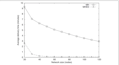
4.2.3 Delivery time

In terms of hop count, MH performs better than ED and MHED. When delivery time is considered, the strong advantage of earliest delivery methods are realized. Figures 17 and 18 show average delivery times for differ-ent network sizes. Note that ED results are omitted from the figures because they are the same as MHED results in terms of delivery time.

(15)

Fig. 15Average path length to destination in a 100 node network under Scenario 1

at best. By having 1.8 times (1.6 hops) longer routes than MH, MHED achieves delivery 7.5 times (14.2 min) faster than MHED, on the average. The delivery time differ-ence increases to more than 50 times when we consider networks larger than 50 nodes.

In Scenario 2, MHED message delivery is at most tens of seconds for networks with more than 20 nodes. The MH method performs relatively better than in Scenario 1, delivering messages in just under 3 min for the largest net-work. Using MHED, routes are 1.4 times (0.7 hops) longer

(16)

Fig. 17Average delivery time of a packet in a network withdensity=0.2 under Scenario 1

than MH routes, whereas MHED delivery is 13.2 times (4.7 min) faster.

An important conclusion so far is that MHED deliv-ers messages quite fast in a network with periodic connections, while minimizing the transmission count

(number of hops). This approach leads to practical benefits. Consider a network consisting of battery-constrained devices. These devices need to save energy by employing sleep/wake schedules, and by transmit-ting as little as possible. If the contact and schedule

(17)

information is known by the whole network, impor-tant gains in battery life are achievable with low-delay communications.

4.2.4 Routing tree stability

We define routing tree stability as the tendency of the paths to destinations to remain the same at successive time intervals. Figures 19 and 20 present routing tree stability for different network sizes. The MH routes are independent of time to a great extent, since the algorithm chooses routes in a hop-count-first manner. The differ-ence in routes is only due to preferring earlier routes among routes with the minimum number of hops. This method results in a higher retention of routes, compared to other methods.

For two reasons, MHED routes are more stable than ED routes. First, MHED routes are shorter in hop count, therefore, are less likely to change from time to time than a path with more hops. Second, MHED routes prefer paths with later delivery times at the beginning of a path, because the algorithm does not make greedy decisions about delivery time.

Although routing tree stability is a metric distinguish-ing among proposed routdistinguish-ing methods, it does not provide any practical benefits because routes need to be calcu-lated at every time unit. A time unit is defined as the finest granularity of time in which connection durations are delineated. In our experiments, we used a time unit of 1 min.

We cannot know for sure whether routes have changed before calculating them. Calculating routes at every time unit could be tedious, but fortunately, we do not need to do this unless we need to route a packet. Therefore, the routing calculation can be performed depending on which occurs later: a time unit passes or a packet to be routed arrives. Indeed, the exact route that a packet will follow is known when the packet is generated at the source. We can use source routing to avoid reculations at each hop. With source routing, routing cal-culations are done only when a packet is generated. If the packet generation rate is faster than one per time unit, a single route calculation suffices for each time unit.

5 Conclusion

The MHED routing algorithm achieves earliest delivery, as ED and epidemic routing do, while routing messages over the minimum number of hops, therefore achiev-ing the minimum number of transmissions. Simulation results verify that MHED finds shorter routes than ED. The advantage of MHED over ED increases for increas-ing network size and decreasincreas-ing density. These properties make MHED routing suitable for DTNs with periodic connections.

Our routing algorithms address periodic connections. In our most detailed connection model, a period con-sists of a connection and a following disconnection, each of certain durations. It is possible to extend this

(18)

Fig. 20Routing tree stability for network withdensity₌0.2dunder Scenario 2

model to super-periods that consist of a cycle of multiple periods with different properties. Super-periods would be useful when connection periods arise due to node availability or sleep schedules. With little modification, our algorithms are capable of routing in such situ-ations, though, for practicality, we need methods to extract and disseminate super-period information from schedules. We are considering super-periods and their application to wireless sensor networks as a future work.

An extension to this study is to apply the MHED rout-ing algorithm to non-scheduled periodic connections, in which connection and disconnection times are not known in advance. Future contact times could be estimated by observing past connection patterns, and routing algo-rithms could be used accordingly.

In this work, we have abstracted from the mobility and have focused on connections. Another future work idea is the application of presented connection models and routing algorithms to different mobility models.

Competing interests

The authors declare that they have no competing interests.

Acknowledgements

This work is supported by TUBITAK (The Scientific and Technological Research Council of Turkey) in part with project 113E274.

Received: 21 February 2015 Accepted: 16 July 2015

References

1. K Fall, inSIGCOMM ‘03: Proceedings of the Conference on Applications,

Technologies, Architectures, and Protocols for Computer Communications. A

delay-tolerant network architecture for challenged internets (ACM, New York, 2003), pp. 27–34. doi:10.1145/863955.863960

2. B Cohen, BitTorrent Protocol (2001). http://bittorrent.org

3. X Sun, Q Yu, R Wang, Q Zhang, Z Wei, J Hu, A Vasilakos, Performance of dtn protocols in space communications. Wirel. Netw.19(8), 2029–2047 (2013). doi:10.1007/s11276-013-0582-0

4. AV Vasilakos, Y Zhang, T Spyropoulos,Delay tolerant networks: protocols

and applications, 1st edn. (CRC Press, Inc., Boca Raton, 2011)

5. CE Perkins, EM Royer, inMobile Computing Systems and Applications, 1999.

Proceedings. WMCSA ‘99. Second IEEE Workshop On. Ad-hoc on-demand

distance vector routing (IEEE Computer Society Washington, DC, USA, 1999), pp. 90–100. doi:10.1109/MCSA.1999.749281

6. T Clausen, P Jacquet, Optimized link state routing protocol (OLSR), 1–75 (2003). doi:http://dx.doi.org/10.17487/RFC362610.17487/RFC3626 7. S Jain, K Fall, R Patra, inSIGCOMM ‘04: Proceedings of the Conference on

Applications, Technologies, Architectures, and Protocols for Computer

Communications. Routing in a delay tolerant network (ACM, New York,

2004), pp. 145–158. doi:10.1145/1015467.1015484

8. P Li, S Guo, S Yu, AV Vasilakos, inINFOCOM, 2012 Proceedings IEEE. Codepipe: An opportunistic feeding and routing protocol for reliable multicast with pipelined network coding (IEEE Communications Society New York, NY, USA, 2012), pp. 100–108.

doi:10.1109/INFCOM.2012.6195456

9. T Spyropoulos, R Rais, T Turletti, K Obraczka, A Vasilakos, Routing for disruption tolerant networks: taxonomy and design. Wirel. Netw.16(8), 2349–2370 (2010). doi:10.1007/s11276-010-0276-9

10. I Woungang, SK Dhurandher, A Anpalagan, AV Vasilakos,Routing in

opportunistic networks. (Springer, Springer Science+Business Media New

York, 2013)

11. A Vahdat, D Becker,Epidemic routing for partially-connected ad hoc

networks. Department of Computer Science, Duke University, (Durham,

North Carolina, NC, USA, 2000). http://www.cs.duke.edu/techreports/ 2000/2000-06.ps

(19)

Symposium on Principles of Distributed Computing. Epidemic algorithms for replicated database maintenance (ACM, New York, 1987), pp. 1–12. doi:10.1145/41840.41841

13. A Lindgren, A Doria, O Schelén, Probabilistic routing in intermittently connected networks. SIGMOBILE Mob Comput. Commun. Rev.7(3), 19–20 (2003). doi:10.1145/961268.961272

14. T Spyropoulos, K Psounis, CS Raghavendra, in2004 First Annual IEEE Communications Society Conference on Sensor and Ad Hoc

Communications and Networks, IEEE SECON 2004. Single-copy routing in

intermittently connected mobile networks (IEEE Communications Society New York, NY, USA, 2004), pp. 235–244

15. V Conan, J Leguay, T Friedman, Fixed point opportunistic routing in delay tolerant networks. IEEE J. Sel. Areas Commun.26(5), 773–782 (2008). doi:10.1109/JSAC.2008.080604

16. T Spyropoulos, K Psounis, CS Raghavendra, inWDTN ‘05: Proceedings of the

ACM SIGCOMM Workshop on Delay-tolerant Networking. Spray and wait: an

efficient routing scheme for intermittently connected mobile networks (ACM, New York, 2005), pp. 252–259. doi:10.1145/1080139.1080143 17. T Spyropoulos, K Psounis, CS Raghavendra, inProceedings of the Fifth IEEE

International Conference on Pervasive Computing and Communications

Workshops. Spray and focus: Efficient Mobility-assisted Routing for

Heterogeneous and Correlated Mobility (IEEE Computer Society Washington, DC, USA, 2007), pp. 79–85. doi:10.1109/PERCOMW.2007.108 18. SC Nelson, M Bakht, R Kravets, inINFOCOM 2009, IEEE. Encounter-based

routing in DTNs (IEEE Communications Society New York, NY, USA, 2009), pp. 846–854. doi:10.1109/INFCOM.2009.5061994

19. Y-S Yen, H-C Chao, R-S Chang, A Vasilakos, Flooding-limited and multi-constrained qos multicast routing based on the genetic algorithm for {MANETs}. Math. Comput. Model.53(11–12), 2238–2250 (2011). Recent Advances in Simulation and Mathematical Modeling of Wireless Networks

20. AT Prodhan, R Das, H Kabir, GC Shoja, TTL based routing in opportunistic networks. J. Netw. Comput. Appl.34(5), 1660–1670 (2011). Dependable Multimedia Communications: Systems, Services, and Applications 21. Z Yang, Q Zhang, R Wang, H Li, A Vasilakos, On storage dynamics of space

delay/disruption tolerant network node. Wirel. Netw.20(8), 2529–2541 (2014). doi:10.1007/s11276-014-0756-4

22. S Merugu, M Ammar, E Zegura,Routing in space and time in networks with predictable mobility. Technical report, College of Computing, Georgia

Institute of Technology, (Atlanta, Georgia, GA, USA, 2004). http://hdl.

handle.net/1853/6492

23. C Liu, J Wu, inMobiHoc ‘07: Proceedings of the 8th ACM International

Symposium on Mobile Ad Hoc Networking and Computing. Scalable routing

in delay tolerant networks (ACM, New York, 2007), pp. 51–60. doi:10.1145/1288107.1288115

24. C Liu, J Wu, inMobiHoc ‘09: Proceedings of the Tenth ACM International

Symposium on Mobile Ad Hoc Networking and Computing. An optimal

probabilistic forwarding protocol in delay tolerant networks (ACM, New York, 2009), pp. 105–114. doi:10.1145/1530748.1530763

25. C Liu, J Wu, inProceedings of the 9th ACM International Symposium on

Mobile Ad Hoc Networking and Computing.MobiHoc ‘08. Routing in a

cyclic mobispace (ACM, New York, 2008), pp. 351–360. doi:10.1145/1374618.1374665

26. A Dvir, AV Vasilakos, Backpressure-based routing protocol for dtns. SIGCOMM Comput. Commun. Rev.41(4), 405–406 (2010)

27. H Dubois-Ferriere, M Grossglauser, M Vetterli, inProceedings of the 4th ACM International Symposium on Mobile Ad Hoc Networking & Computing. MobiHoc ‘03. Age matters: efficient route discovery in mobile ad hoc networks using encounter ages (ACM, New York, 2003), pp. 257–266. doi:10.1145/778415.778446

28. EM Daly, M Haahr, inProceedings of the 8th ACM International Symposium

on Mobile Ad Hoc Networking and Computing.MobiHoc ‘07. Social network

analysis for routing in disconnected delay-tolerant manets (ACM, New York, 2007), pp. 32–40. doi:10.1145/1288107.1288113. http://doi.acm.org/ 10.1145/1288107.1288113

29. P Hui, J Crowcroft, E Yoneki, inProceedings of the 9th ACM International

Symposium on Mobile Ad Hoc Networking and Computing.MobiHoc ‘08.

Bubble rap: social-based forwarding in delay tolerant networks (ACM, New York, 2008), pp. 241–250. doi:10.1145/1374618.1374652 30. E Bulut, SC Geyik, BK Szymanski, inProceedings of the 2010 IEEE

International Symposium on A World of Wireless, Mobile and Multimedia

Networks (WoWMoM).WOWMOM ‘10. Conditional shortest path routing

in delay tolerant networks (IEEE Computer Society Washington, DC, 2010), pp. 1–6. doi:10.1109/WOWMOM.2010.5534960

31. Q Ayub, S Rashid, MSM Zahid, AH Abdullah, Contact quality based forwarding strategy for delay tolerant network. J. Netw. Comput. Appl.

39(0), 302–309 (2014). doi:10.1016/j.jnca.2013.07.011

32. M Youssef, M Ibrahim, M Abdelatif, L Chen, AV Vasilakos, Routing metrics of cognitive radio networks: a survey. IEEE Commun. Surv. Tutorials.16(1), 92–109 (2014). doi:10.1109/SURV.2013.082713.00184

33. EPC Jones, L Li, PAS Ward, inWDTN ‘05: Proceedings of the ACM SIGCOMM

Workshop on Delay-tolerant Networking. Practical routing in delay-tolerant

networks (ACM, New York, 2005), pp. 237–243. doi:10.1145/1080139.1080141

34. Y Zeng, K Xiang, D Li, A Vasilakos, Directional routing and scheduling for green vehicular delay tolerant networks. Wirel. Netw.19(2), 161–173 (2013). doi:10.1007/s11276-012-0457-9

35. TH Cormen, CE Leiserson, RL Rivest, C Stein,Introduction to algorithms, 2nd revised edn. (The MIT Press, Cambridge, Massachusetts, MA, USA, 2001)