Filter regularization method for a time fractional inverse advection–dispersion problem

(1)

R E S E A R C H

Open Access

Filter regularization method for a

time-fractional inverse advection–dispersion

problem

Songshu Liu

1

_{and Lixin Feng}

2*

*_{Correspondence:}

[email protected] 2_{Heilongjiang Provincial Key} Laboratory of the Theory and Computation of Complex Systems, School of Mathematical Sciences, Heilongjiang University, Harbin, P.R. China

Full list of author information is available at the end of the article

Abstract

A ﬁlter regularization method is developed to solve a time-fractional inverse

advection–dispersion problem, which is based on the modiﬁed ‘kernel’ idea. Proofs of convergence are given under both priori and posteriori regularization parameter choice rules. Numerical examples are presented to illustrate the eﬀectiveness of the proposed algorithm.

Keywords: Inverse problem; Time-fractional advection–dispersion equation; Filter regularization method; A priori parameter choice; A posteriori parameter choice

1 Introduction

In the last few decades, many problems in finance [1, 2], physics [3–6], control theory [7], hydrology [8,9] and viscoelasticity [10] were modeled mathematically by fractional partial differential equations. The biggest important advantage of using fractional partial differential equations in mathematical modeling is their non-local property in the sense that the next state of the system depends not only upon its current state but also upon all of its proceeding states. The fractional-order models are more adequate than the integral-order models to describe the memory and hereditary properties of different substances [11–17].

In practical physical applications, Brownian motion, the diffusion with an additional velocity field and diffusion under the influence of a constant external force field are both modeled by the advection–dispersion equation [18]. However, the advection–dispersion equation is not suitable for anomalous diffusion, i.e., the fractional generalization may be different for the advection case and the transport in an external force field [19]. A straight-forward extension of the continuous time random walk (CTRW) model leads to a frac-tional advection–dispersion equation. The time-fracfrac-tional advection–dispersion equa-tion is obtained by replacing the time-derivative in the advecequa-tion–dispersion equaequa-tion by a generalized derivative of orderαwith 0 <α≤1 and can be used to simulate contaminant transport in porous media [20]. Direct problems for time-fractional advection–dispersion equations have been studied extensively in recent years [21–24]. By contrast, little has been done on the inverse problems for time-fractional advection–dispersion equations.

(2)

In this paper, the inverse problem of time-fractional advection–dispersion equation is given by

⎧ ⎪ ⎪ ⎪ ⎪ ⎪ ⎨ ⎪ ⎪ ⎪ ⎪ ⎪ ⎩

0Dαtu(x,t) +bux(x,t) =auxx(x,t), x> 0,t> 0,

u(x, 0) = 0, x≥0,

u(x,t)|x→∞ bounded, t≥0,

u(1,t) =g(t), t≥0,

(1.1)

whereuis the solute concentration, the constantsa(a> 0) andb(b≥0) represent the dis-persion coefficient and the average fluid velocity, respectively. The time-fractional deriva-tive0Dαtu(x,t) is the Caputo fractional derivative of orderα(0 <α≤1) defined by [11]

0Dαtu(x,t) = ⎧ ⎨ ⎩

1 Γ(1–α)

t

0 ∂u(x,s)

∂s ds

(t–s)α, 0 <α< 1,

∂u(x,t)

∂t , α= 1.

The problem is to detect the temperature for 0≤x< 1 by means of the current temper-ature measurement atx= 1. It is well known that this problem is ill-posed, since the small errors in the input data may cause large errors in the output solution.

Recently, time-fractional inverse diffusion problems have been considered by some au-thors; see [25–29]. Although there are many papers on time-fractional inverse diffusion problems, we only find a few results on inverse problems for time-fractional advection– dispersion equations. Zheng and Wei [30,31] applied the spectral regularization method and the modified equation method to a time-fractional inverse advection–dispersion problem, respectively. Following the work of [30,31], Zhao et al. [32] used an optimal fil-tering method to deal with a time-fractional inverse advection–dispersion problem. How-ever, the theoretical studies in the literature [30–32] were only based on a priori regular-ization parameter choice rule. The main aim of this present work is to present a filter reg-ularization method and prove the convergence estimates under both priori and posteriori regularization parameter choice rules. The advantages of the proposed approach over the other existing results available in the literature [30–32] are demonstrated in Remark3.5, Remark3.6, Remark3.8and Remark4.6in detail.

The idea of filter regularization method by modified ‘kernel’ is very simple and natural, since the ill-posedness of time-fractional inverse advection–dispersion problem is caused by the high frequency components of the ‘kernel’, the ‘kernel’ function can be modified. As long as the modified ‘kernel’ function satisfies som certain properties, a new regularization method can be established. In addition, the modified ‘kernel’ idea has been used to deal with several ill-posed problems [33–36].

This paper consists of six sections. Section2states the ill-posedness of the problem and presents a ﬁlter regularization method. In Sects.3and4, the error estimates are proved under both prior and posterior regularization parameter choice rules. Numerical experi-ments are performed in Sect.5. A brief conclusion is given in Sect.6.

2 Ill-posedness of the problem and a ﬁlter regularization method

(3)

denotes theL2_{-norm, i.e.,}

The Fourier transform of the functionf(t) is written as

f(ξ) =√1

Taking the Fourier transform to (1.1) with respect tot, one can easily get the solution of problem (1.1) in the frequency domain

u(x,ξ) =e(1–x)k(ξ)g(ξ), (2.1)

(4)

an error, and it satisﬁes

gδ₍_t_{) –}_g₍_t₎_≤_δ, _(2.4)

whereδ> 0 is a noise level. This mean a small error for the measured datagδ₍_t_{) will be}

am-plified infinitely by the factore(1–x)Aand destroy the solution of problem (1.1). Therefore, the time-fractional inverse advection–dispersion problem is severely ill-posed and some regularization methods are needed. Thus, a filter regularization method to solve problem (1.1) is presented in this paper.

To regularize the problem, our aim is to replace the terme(1–x)A _{by another term. For} this purpose, a regularized solution in frequency space is deﬁned as follows:

uβ,δ(x,ξ) = e

(1–x)k(ξ)

1 +β|ek(ξ)|g δ

(ξ), (2.5)

or equivalently

uβ,δ₍_x_,_t_{) =} _√1

2π

∞

–∞

eiξt e(1–x)k(ξ) 1 +β|ek(ξ)|g

δ_(ξ₎_d_ξ_. _(2.6)

In the following section, the error estimates between the regularized solutionuβ,δ₍_x_,_t₎

and the exact solutionu(x,t) will be proved under both prior and posterior regularization parameter choice rules.

3 Prior choice rule and error estimate

In this section, theL2_{-estimate and}_Hp_{-estimate are discussed under a prior regularization} parameter choice rule, respectively. Before obtaining the main theorems, some auxiliary lemmas ﬁrstly are given.

Lemma 3.1([31]) If x∈[0, 1),and k(ξ)is given by(2.3),then the following inequality holds: k(ξ) ≤|ξ|

α 2

√

a.

Lemma 3.2([37]) Let0 <x<a, 0 <μ< 1,then

sup

η≥0 eηx 1 +μeηa ≤μ

–x_a_.

3.1 L2_-Estimate

Theorem 3.3 Suppose that u(x,·)is the exact solution of problem(1.1)and uβ,δ₍_x_,_·₎_{is the}

ﬁlter regularized solution of problem(1.1).Let the assumption(2.4)and the prior condition

u(0,·) ≤E hold.If the regularization parameterβis selected by

β=δ

E, (3.1)

then we have the following error estimate:

(5)

Proof Due to Parseval’s formula and the triangle inequality, we have

According to Lemma3.2, it is obvious that

C(ξ) =sup

Combining the formulas (3.3)–(3.5), it follows that

uβ,δ(x,·) –u(x,·)≤Eβx+δβx–1, (3.6)

using Eq. (3.1), the error estimate (3.2) is obtained.

Remark3.4 From (3.2), it is clear that a Hölder-type estimate in the interval 0 <x< 1 is obtained. However, the error estimate atx= 0 cannot be obtained. In order to obtain the error estimate atx= 0, a stronger prior bound is introduced as follows:

u(0,·)_Hp≤E. (3.7)

(6)

Remark 3.6 In [31], the authors regularize the time-fractional inverse advection– dispersion problem and derive the error estimate

uβ,δ(x,·) –u(x,·)≤ε1+ C2·E

(lnE_δ)4.

Thus, the convergence rate in this work is better than the one in [31].

3.2 Hp_-Estimate

Theorem 3.7 Suppose that u(0,·)is the exact solution of problem(1.1)and uβ,δ_(0,_·₎_{is the}

ﬁlter regularized solution of problem(1.1).Let the assumption(2.3)and the prior condition

u(0,·)Hp≤E hold.If the regularization parameterβis selected by

then we have the following error estimate:

uβ,δ(0,·) –u(0,·)≤δ12_E12 ₊_E_max

Proof Using the analogous technique of Theorem3.3, it is evident that

uβ,δ(0,·) –u(0,·)=uβ,δ(0,·) –u(0,·)

≤uβ,δ_(0,_·_{) –}_uβ_(0,_·₎₊_uβ_(0,_·_{) –}_u_(0,_·₎_. _(3.10)

For the ﬁrst term on the right-hand side of (3.10), the following inequality holds:

uβ,δ(0,·) –uβ(0,·)≤δsup

whereEis the prior bound.

(7)

Then the following inequality can be obtained:

uβ(0,·) –u(0,·)≤Emax

ln1 β

–p ,β1–

α 2√a

. (3.13)

Taking into account (3.8), (3.10), (3.11), (3.12) and (3.13), the error estimate (3.9) is

ob-tained.

Remark3.8 In [30–32], the convergence estimates have been obtained under a prior reg-ularization parameter choice rule. However, in practical computations, such choices do not work well for all cases. Therefore, it is better to provide a posterior regularization parameter choice rule. In the next section, this topic is considered.

4 Posterior choice rule and error estimate

This section presents a posterior regularization parameter choice by Morozov’s discrep-ancy principle. Choose the regularization parameterβas the solution of the equation

_{1 +}_β1_|_ek(ξ)|g

δ_{(ξ) –}_gδ_(ξ₎₌_{τ δ,} _(4.1)

whereτ > 1 is a constant andβ denotes the regularization parameter. To establish exis-tence and uniqueness of solution for Eq. (4.1), the following lemmas are needed.

Lemma 4.1 Letρ(β) :=₁₊_β_|1_ek(ξ)_|gδ(ξ) –gδ(ξ),if0 <τ δ<gδ(ξ),then

(a) ρ(β)is a continuous function; (b) limβ→0ρ(β) = 0;

(c) limβ→+∞ρ(β) =gδ;

(d) ρ(β)is a strictly increasing function.

The proof is very easy and we omit it here.

Remark4.2 From Lemma4.1, it is known that there exists a unique solutionβsatisfying Eq. (4.1).

Lemma 4.3 Ifβis the solution of Eq. (4.1),then the following inequality holds:

1

1 +β|ek(ξ)_|g δ

(ξ) –g(ξ)≤(τ+ 1)δ. (4.2)

Proof Due to the triangle inequality and Eq. (4.1), we have

_{1 +}_β1_|_ek(ξ)_|g

δ_(ξ_{) –}_g_(ξ)

≤ 1

1 +β|ek(ξ)_|g δ

(ξ) –gδ(ξ)+gδ(ξ) –g(ξ)

≤(τ+ 1)δ. (4.3)

(8)

Lemma 4.4 Ifβis the solution of Eq. (4.1),the following inequality also holds:

β–1≤ E

(τ– 1)δ. (4.4)

Proof Due to the triangle inequality and Eq. (4.1), we have

τ δ = 1

Now, the main theorem is given as follows.

Theorem 4.5 Suppose that the prior conditionu(0,·) ≤E and the assumption(2.4)hold,

and there existsτ> 1such that0 <τ δ<gδ_._{The regularization parameter}_β_{> 0}_{is chosen}

by Morozov’s discrepancy principle(4.1).Then the following convergence estimate holds:

uβ,δ(x,·) –u(x,·)≤

Proof Due to the Parseval formula and Lemma4.3, we have

(9)

· ∞

Using Lemma4.4, it follows that

uβ,δ(x,·) –u(x,·)2≤δβ–1+E2(1–x)·(τ+ 1)δ2x

Therefore, the conclusion of the theorem can be obtained directly from (4.8).

Remark4.6 Obviously, Ifα= 1, the problem (1.1) naturally corresponds to the standard inverse advection–dispersion problem [38]. Ifα= 1 andb= 0, the problem (1.1) corre-sponds to the classical inverse heat conduction problem [39]. Ifb= 0, the problem (1.1) corresponds to the time-fractional inverse diﬀusion problem [40]. Thus, the results in the paper are valid for these special problems.

5 Numerical examples

In this section, three numerical examples are presented to illustrate the behavior of the proposed method. In our numerical experiment, we seta= 1 andb= 1 in (1.1).

The numerical examples are constructed in the following way. First, the initial data

u(0,t) =f(t) of time-fractional advection–dispersion problem is presented atx= 0, and the functionu(1,t) =g(t) is computed by solving a direct problem, which is a well-posed problem. Second, a randomly distributed perturbation to the data function obtaining vec-torgδ₍_t_{) is added, i.e.,}

(10)

Here, the function “randn(·)” generates arrays of random numbers whose elements are normally distributed with mean 0, variance σ2 = 1 and standard deviationσ = 1, “randn(size(g))” returns array of random entries that is the same size asg, the magni-tudeindicates a relative noise level. Here, the total noiseδcan be measured in the sense of the root mean square error according to

δ:=gδ–g_l2=

Third, the regularized solution is obtained by solving the inverse problem. Finally, the regularized solution is compared with the exact solution.

In the experiments under the prior regularization parameter choice rule, the regular-ization parameterβis chosen by (3.1), and in the experiments under the posterior regu-larization parameter choice rule, the reguregu-larization parameterβ is chosen by (4.1) with τ = 1.1.

Example5.1 Consider a smooth function

f(t) = 4sin(2πt). (5.3)

Example5.2 Consider a piecewise smooth function

f(t) =

Example5.3 Consider the following discontinuous function:

f(t) =

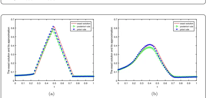
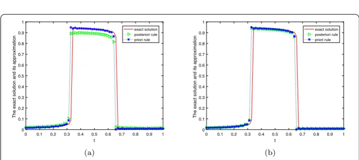
Figures1,3and5show the comparison between prior and posterior methods for dif-ferentαfor Examples5.1,5.2,5.3, respectively. Figures2,4and6show the comparison between prior and posterior methods for diﬀerent for Examples5.1,5.2,5.3, respec-tively.

(11)

Figure 1The comparison of the exact solution and its approximation solution for= 0.01 atx= 0.8 with Example5.1, (a)α= 0.1, (b)α= 0.7

Figure 2The comparison of the exact solution and its approximation solution forα= 0.3 atx= 0.1 with Example5.1, (a)= 0.01, (b)= 0.001

6 Conclusion

(12)

and Morozov’s discrepancy principle. The numerical examples verify the eﬃciency and accuracy of the proposed computational method.

(13)

prob-lems. On the other hand, the proposed method can be extended to the case with time-dependent coeﬃcient. Towards this end, more vigorous investigations are needed in the future.

Funding

This work was partially supported by National Natural Science Foundation of China (11871198), the Fundamental Research Funds for the Universities of Heilongjiang Province Heilongjiang University Special Project (RCYJTD201804), the National Science Foundation of Hebei Province (A2017501021) and the Fundamental Research Funds of the Central Universities (N182304024).

Competing interests

The authors have declared that no competing interests exist.

Authors’ contributions

The main idea of this paper was proposed by LF. SL prepared the manuscript initially and performed all the steps of the proofs in the research. All authors read and approved the ﬁnal manuscript.

Author details

1_{School of Mathematics and Statistics, Northeastern University at Qinhuangdao, Qinhuangdao, P.R. China.}2_Heilongjiang

Provincial Key Laboratory of the Theory and Computation of Complex Systems, School of Mathematical Sciences, Heilongjiang University, Harbin, P.R. China.

Publisher’s Note

Springer Nature remains neutral with regard to jurisdictional claims in published maps and institutional aﬃliations.

Received: 14 March 2019 Accepted: 23 May 2019

References

1. Roberto, M., Scalas, E., Mainardi, F.: Waiting-times and returns in high frequency ﬁnancial data: an empirical study. Physica A314, 171–180 (2002)

2. Sabatelli, L., Keating, S., Dudley, J., Richmond, P.: Waiting time distributions in ﬁnancial markets. Eur. Phys. J. B27, 273–275 (2002)

3. West, B., Bologna, M., Grigolini, P.: Physical of Fractal Operators. Springer, New York (2003) 4. Hilfer, R.: Application of Fractional Calculus in Physics. World Scientiﬁc, Singapore (2000)

5. Xu, W., Sun, H., Chen, W., Chen, H.: Transport properties of concrete-like granular materials interacted by their microstructures and particle components. Int. J. Mod. Phys. B32, 1840011 (2018)

6. Sun, H., Zhang, Y., Wei, S., Zhu, J., Chen, W.: A space fractional constitutive equation model for non-Newtonian ﬂuid ﬂow. Commun. Nonlinear Sci. Numer. Simul.62, 407–417 (2018)

7. Mechado, J.A.T.: Discrete time fractional-order controllers. Fract. Calc. Appl. Anal.4, 47–66 (2001)

8. Baeumer, B., Meerschaert, M.M., Benson, D.A., Wheatcraft, S.W.: Subordinate advection–dispersion equation on contaminant transport. Water Resour. Res.37, 1543–1550 (2001)

9. Schumer, R., Benson, D.A., Meerschaert, M.M., Baeumer, B.: Multiscaling fractional advection–dispersion equations and their solutions. Water Resour. Res.39, 1022–1032 (2003)

10. Bagley, R.L., Torvik, P.J.: A theoretical basis for the application of fractional calculus to viscoelasticity. J. Rheol.27, 201–210 (1983)

11. Podlubny, I.: Fractional Diﬀerential Equations. Acadmic Press, San Diego (1999)

12. Hajipour, M., Jajarmi, A., Baleanu, D., Sun, H.: On an accurate discretization of a variable-order fractional reaction-diﬀusion equation. Commun. Nonlinear Sci. Numer. Simul.69, 119–133 (2019)

13. Baleanu, D., Jajarmi, A., Asad, J.H.: Classical and fractional aspects of two coupled pendulums. Rom. Rep. Phys.71, 103 (2019)

14. Meng, R., Yin, D., Drapaca, C.S.: Variable-order fractional description of compression deformation of amorphous glassy polymers. Comput. Mech. (2019).https://doi.org/10.1007/s00466-018-1663-9

15. Baleanu, D., Jajarmi, A., Hajipour, M.: On the nonlinear dynamical systems within the generalized fractional derivatives with Mittag-Leﬄer kernel. Nonlinear Dyn.94, 397–414 (2018)

16. Baleanu, D., Sajjadi, S.S., Jajarmi, A., Asad, J.H.: New features of the fractional Euler–Lagrange equations for a physical system within non-singular derivative operator. Eur. Phys. J. Plus134, 181 (2019)

17. Baleanu, D., Jajarmi, A., Bonyah, E., Hajipour, M.: New aspects of poor nutrition in the life cycle within the fractional calculus. Adv. Diﬀer. Equ.2018, 230 (2018)

18. Khalifa, M.E.: Some analytical solutions for the advection–dispersion equation. Appl. Math. Comput.139, 299–310 (2003)

19. Metzler, R., Klafter, J.: The random walk’s guide to anomalous diﬀusion: a fractional dynamics approach. Phys. Rep. 339, 1–77 (2000)

20. Bear, J.: Hydraulics of Groundwater. McGraw-Hill, New York (1979)

21. Meerschaert, M.M., Tadjeran, C.: Finite diﬀerence approximations for fractional advection–dispersion ﬂow equations. J. Comput. Appl. Math.172, 65–77 (2004)

22. Wang, K., Wang, H.: A fast characteristic finite difference method for fractional advection-diffusion equations. Adv. Water Resour.34, 810–816 (2011)

(14)

24. Huang, F., Liu, F.: The time fractional diﬀusion equation and the advection–dispersion equation. ANZIAM J.46, 317–330 (2005)

25. Cheng, J., Nakagawa, J., Yamamoto, M., Yamazaki, T.: Uniqueness in an inverse problem for a one-dimensional fractional diﬀusion equation. Inverse Probl.25, 115002 (16 pp.) (2009)

26. Zhang, Y., Xu, X.: Inverse source problem for a fractional diﬀusion equation. Inverse Probl.27, 035110 (12 pp.) (2011) 27. Jin, B., Rundell, W.: An inverse problem for a one-dimensional time-fractional diﬀusion problem. Inverse Probl.28,

075010 (19 pp.) (2012)

28. Liu, J.J., Yamamoto, M.: A backward problem for the time-fractional diﬀusion equation. Appl. Anal.89, 1769–1788 (2010)

29. Li, G., Zhang, D., Jia, X., Yamamoto, M.: Simultaneous inversion for the space-dependent diffusion coefficient and the fractional order in the time-fractional diffusion equation. Inverse Probl.29, 065014 (36 pp.) (2013)

30. Zheng, G.H., Wei, T.: Spectral regularization method for the time fractional inverse advection–dispersion equation. Math. Comput. Simul.81, 37–51 (2010)

31. Zheng, G.H., Wei, T.: A new regularization method for the time fractional inverse advection–dispersion problem. SIAM J. Numer. Anal.49, 1972–1990 (2011)

32. Zhao, J.J., Liu, S.S.: An optimal ﬁltering method for a time-fractional inverse advection–dispersion problem. J. Inverse Ill-Posed Probl.24, 51–58 (2016)

33. Qian, Z., Fu, C.L.: Regularization strategies for a two-dimensional inverse heat conduction problem. Inverse Probl.23, 1053–1068 (2007)

34. Qian, Z., Fu, C.L., Feng, X.L.: A modiﬁed method for high order numerical derivatives. Appl. Math. Comput.182, 1191–1200 (2006)

35. Zhang, Z.Q., Ma, Y.J.: A modiﬁed kernel method for numerical analytic continuation. Inverse Probl. Sci. Eng.21, 840–853 (2013)

36. Liu, S.S., Feng, L.X.: A posteriori regularization parameter choice rule for a modiﬁed kernel method for a time-fractional inverse diﬀusion problem. J. Comput. Appl. Math.353, 355–366 (2019)

37. Feng, X.L., Ning, W.T., Qian, Z.: A quasi-boundary-value method for a Cauchy problem of an elliptic equation in multiple dimensions. Inverse Probl. Sci. Eng.22, 1045–1061 (2014)

38. Qian, Z., Fu, C.L., Xiong, X.T.: A modiﬁed method for a non-standard inverse heat conduction problem. Appl. Math. Comput.180, 453–468 (2006)

39. Berntsson, F.: A spectral method for solving the sideways heat equation. Inverse Probl.15, 891–906 (1999) 40. Xiong, X.T., Gao, H., Liu, X.: An inverse problem for a fractional diﬀusion equation. J. Comput. Appl. Math.236,