Sub Nyquist sampling for short pulses with Gabor frames

R E S E A R C H

Open Access

Sub-Nyquist sampling for short pulses with

Gabor frames

Cheng Wang

1*

, Ying Wang

2

, Peng Chen

3

, Chen Meng

1

, Xiangjun Song

3

and Wanling Li

3

Abstract

For analog signals comprised of several, possibly overlapping, finite duration pulses with unknown shapes and time positions, an efficient sub-Nyquist sampling systems is based on Gabor frames. To improve the realizability of this sampling system, we present alternative method for the case that Gabor windows are high order exponential

reproducing windows. Then, the time translation element could be realized with exponential filters. In this paper, we also construct the measurement matrix and prove that it has better coherence than Fourier matrix. Besides, for satisfying restricted isometry property (RIP), we reduce the row number and the sparsity by stretching windows and raising E-spline smoothness order. We deduce the signal reconstruction error bound, proving that appropriate selection of the stretching factor and smoothness order guarantees low reconstruction error. At last, we also provide the error bound in presence of noise, showing that the sampling scheme holds nice robustness with high Gabor frames redundancy.

Keywords:Compressed sensing, Gabor frames, Exponential reproducing windows, Sub-Nyquist sampling, Xampling

1 Introduction

Sub-Nyquist sampling, which can acquire signals even at very low sampling rate and yet maintain high approxima-tion precision, has been developed over the past years to process certain signal models [1]. Unlike the traditional sub-Nyquist methods such as demodulation, under sam-pling ADC, and periodic nonuniform samsam-pling, Xamsam-pling originates from CS theory (compressed sensing) and ends up in some less sophisticated front-end hardware [2–5]. Until now, a variety of different applications of Xampling is developed for multipulse signals, such as radar signals [6, 7], ultrasound signals [8], and certain signals prevalent in smart power system [9, 10] and smart city [11, 12]. However, all the applications are based on finite-rate-of-innovation (FRI) signals sampling [13, 14], and the pulse shape should be a priori known. Gabor frame sub-Nyquist sampling is proposed for making up for the weakness of FRI signals sampling and can acquire both location and shape information for multipulse signals [15]. Unlike the FRI signals sampling, which just collects the signal Fourier coefficients and reconstruct original signal with kernel functions, it operates short-time Fourier transform on sig-nal and collects the Gabor time-frequency coefficients.

Structurally, Gabor frame sub-Nyquist sampling scheme gets a little more closer to the time domain edition of modulated wideband converter (MWC) [16], which cuts the frequency domain into many lattices and measures the linear compressive translations [17]. It cuts the time domain with modulated window sequences, namely Gabor frames, and recovers exact time locations and shape with CS algorithms.

We focus here on a class of multipulse signals, which have limited time duration and short pulses with arbi-trary shapes and positions, and may even overlap. The

only parameters assumed are the durationT, the number

Npof pulses, and the maximal widthW. The multipulse

signal, x(t), supported on the interval [−T/2,T/2], which can be expressed as

x tð Þ ¼X

N

n¼1

hnð Þt ; where maxnjsupphnj≤W ð1Þ

Ifϵ_Ω< 1, a signal withϵ_Ω—bandlimited toF= [−Ω/2,Ω/2], named as essential band, is defined as

Z

Fcj^x ifð Þj 2_df

1=2

≤Ω∥x tð Þ∥2 ð2Þ

where ^x ifð Þ denotes the Fourier transform of x(t) and the symbolFcthe complement of the setF.

* Correspondence:[email protected]

1_{Shijiazhuang Mechanical Engineering College, Shijiazhuang 050003, China}

Full list of author information is available at the end of the article

Theoretically, all square-integrable time-limited signals can be well approximated by truncated Gabor series. Under Gabor sampling scheme, the sampling rate equals 1/Tand the sampling number is about only 4μ−1Ω′WNp, whereΩ′

is related to the essential bandwidth of the signal andμ∈(0, 1) is the redundancy of the Gabor frames used for process-ing. The sampling scheme in [15] is demonstrated to possess great reconstruction performance with time domain modu-lation measurement functions constructed by Bernoulli random matrix and Gabor window sequences, such as piecewise spline or B-spline window sequences. Unfortu-nately, there still exists a gap between the theory and prac-tice, because the shifting Gabor windows modulated by random measurement matrix is hard to be realized with simple circuit, and its complexity and synchronization preci-sion also greatly affect the reconstruction performance.

The first and main contribution of this paper is introdu-cing the exponential reproduintrodu-cing windows into Gabor sampling scheme and reducing the time domain modula-tion funcmodula-tions, constructed by appropriately weighted win-dow sequences, to simple exponential functions. The time domain modulation functions of this study can avoid holding complicated function structures and intricate sys-tem functions, which are difficult to realize in real world. Any time domain response function from E-spline system could be defined as exponential reproducing function, the simplest one being E-spline itself [18]. Interestingly, with appropriate weighting coefficients, the exponential repro-ducing window sequences can be synthesized to a simple exponential function. It could be viewed as the impulse re-sponse representation of an exponential filter, which can be carried out with simple passive electric circuit [19, 20]. For this study, we deduced the representation of the filter form of the time domain modulation functions in Gabor sampling scheme and chose the appropriate

E-spline parameter vector α for guaranteeing the

win-dow positive real functions. Then, we constructed the measurement matrix for CS recovery and calculated each entry and proved that such measurement matrix has better coherence than that of DFT matrix. Hence, the measurement matrix satisfies the RIP, making it possible to recover the sparse Gabor coefficient matrix perfectly.

Next, we study the effect of frame window widthWgon

the signal reconstruction performance. In [15], the frame window width is the same as the pulse width of the signal to be measured and the Gabor frames is not quite redun-dant. So the sparsity Sof the Gabor coefficients recovered for signal representation is very small and the column

di-mension to row number ratiorof the measurement matrix

is large enough to result in good RIP. However, to ensure enough sampling channel number in the sampling scheme proposed here, the E-spline smoothness orderNshould not be too small. According to [21], ifNis large, which means

the frame windows are high order exponential reproducing windows, the frames will be very redundant, and so the RIP may be hard to be satisfied [22]. In this study, we find that, for neutralizing the disadvantage caused by the redundancy,

the frame windows widthWgcould be stretched wider to

bring down Sand increase r, enhancing the measurement

matrix RIP. Then, we deduce the signal reconstruction error bound, proving that it is effective for improving signal reconstruction performance.

As a third contribution, we study the robustness of the proposed sampling scheme. We deduce the signal recon-struction error bound with noise injected to the sam-pling scheme. From the error bound representation, we

discover that when N is raised to a bigger number, the

redundancy would be μ≪1, which enables the Gabor

frames to hold good robustness. If the sampling channel numbers are the same, our sampling scheme can sup-press noise better than in [15].

2 Background and problem formulation

2.1 Gabor sampling scheme

For any functions x(t),g(t)∈L2(ℝ), whose modulation

and translation operators are defined as Mblx(t) =

e2πiblt and Takx(t) =x(t−ak), there exist constants 0

<A≤B<∞, making a collection Gðg;a;bÞ ¼ MblTakg tð Þ ¼e2πibltg tð−akÞ;k;l∈ℤ

satisfy

Ajjxjj2_≤X k;l∈ℤ

jhx;MblTakgij2≤Bjjxjj2; ð3Þ

then Gðg;a;bÞ is a Gabor frame. If we define Gabor frame coefficients as zkl=Vgx(ak,bl) =〈x,MblTakg〉, then

signalx(t) can be expanded with Gabor frames as

x¼X

k;l∈ℤ

zk;lMblTakγ ð4Þ

In Eq. (4),γ(t) is the dual window ofg(t) andGðγ;a;bÞ

is the corresponding dual frame. Generally, if g(t) is compactly supported on some interval [−Wg/2,Wg], with a=μWg,b= 1/Wgfor someμ∈(0, 1), the frame operator

takes on the particularly simple formS tð Þ ¼P

k∈ℤ jg t−akð Þj 2_,

and the canonical dual will be γ(t) =bS−1g(t) [23]. In addition, here there exists γ(t)∈S0, where S0is the Segal algebra space, defined as [24]

S0:¼ x∈L2ð Þjℝ k kx S0 ¼ Vφx L1ð_ℝℝ^Þ<∞

ð5Þ

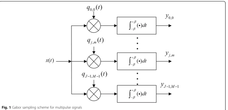
In the sampling scheme, the signal x(t) enters J×M

channels simultaneously. In the (j,m) th channel, x(t) was multiplied by a function qj,m(t) and processed by

an integrator. The structure of the scheme is shown in Fig. 1.

Matusiak and Eldar [15] set Wg=W, and g(t)

essen-tially bandlimited to [−Bg/2,Bg/2]. For some, μ∈(0, 1),

qj,m(t) =wj(t)sm(t) is defined, wherewjð Þ ¼t

XL0

l¼−L0

djle−2πiblt

;smð Þ ¼t

XK0

k¼−K0

cmkg tð−akÞ. Here, K0¼

⌈

TþW_2Wμ

⌉

−1 and L0

¼

⌈

ðΩþB₂ÞW

⌉

−1 , and then the numbers of time and fre-quency shifts are respectively K= 2K0+ 1 and L= 2L0+ 1. The output of the (j,m) th channel is

y_j;m ¼

Z T=2

−T=2

x tð Þq_j;mð Þdtt ¼ X

L0

l¼−L0

djl XK0

k¼−K0

cmkzkl ð6Þ

Equation (6) can be written in the matrix equation as

Y¼DUT_{; withU¼CZ ð7Þ}

For general multipulse signals, matrixD was used only to simplify hardware implementation, but not to reduce sampling rate. Matusiak and Eldar [15] chose matrixDas

D=Ior other full bank matrix withJ≥L, reducing the pri-mary mission of Eq. (7) toU=CZ. Relying on ideas of CS, the signal can be recovered from a small number of sam-ples by exploiting its sparsity. Then, the multipulse signal

x(t) can be recovered according to Eq. (4).

Recovering matrixZis referred to as a multiple

meas-urement vector (MMV) problem [21]. In [15], matrix C

was chosen as Gaussian or Bernoulli random matrices, which have RIP of the order S, if M≥2⌈2μ−1⌉Nlog(K/ 2⌈2μ−1⌉N). The RIP is defined as follows.

For every S-sparse vector x, matrix Φhas the (S,δS

)-restricted isometry property (RIP), if

1−δS

ð Þk kx 2≤kΦxk2≤ð1þδSÞk kx 2 ð8Þ

for the smallest constant δS, which is called restricted

isometry constant (RIC).

2.2 Exponential reproducing windows

An exponential reproducing window is any functiong(t) that, together with its shifted versions, can generate complex exponentials of the formeαnt_{, such as}

X

k∈ℤ

vn;kg tð−kÞ ¼eαnt ð₉Þ

where n= 0, 1,…,N, and αn∈ℂ. The coefficients are

given by representation vn;k¼ Z

−∞ ∞

eαntγð_t−_kÞdt_.

Know-ing that the coefficients vn,k are discrete-time

exponen-tials, we express them in another form

vn;k¼ Z _∞

−∞e

αnt_eαnkγð Þdt_t ¼_eαnk_v

n;0 ð10Þ

The theory relating to the reproduction of exponen-tials derives from the concept of E-splines [18]. A

function with the time domain representation β_α¼eα

rect t−1 2

is called cardinal E-spline of first order. Through convolution of β_α, Nthorder E-splines can be

obtained, e.g., β_αð Þ ¼t β_α1β_α2⋯β_αN

t

ð Þ, whereα = (α1,α2,…,αN), and it can be written in the Fourier

do-main as ^β_αð Þ ¼ω Y N

n¼1 1−eαn−jω

jω−an

. As exponent αn can be

exponents. The functionβαis of compact support, and a

linear combination of its shifted versionsβα(t−k)

repro-duces the exponentialeα. Besides E-splines, any function

g(t) =ψ(t) *βα(t) holds the property of reproducing

expo-nentials in the subspace spanned byfeα1;_eα2;…;_eαNg_.

3 Sampling scheme with exponential reproducing windows

We now present a sampling scheme with exponential re-producing windows that can greatly simplify the time domain transform function sm(t) using the exponential

reproducing property. Primarily, compared with the time duration [−T/2,T/2] set in [15], shifting the time dur-ation to a complete positive scope [0,T], E-splines are generally defined in a positive domain. For short pulse stream, it satisfies thatWNp≪Tand matrixZis sparse.

3.1 Exponential reproducing transform windows

According to Section 2.2, exponential reproducing windows

g(t) =ψ(t) *βα(t) is considered as response to sampling

ker-Then, Gabor window g(t) is compactly supported in

interval [0,Wg]. In this scenario, the lattice parameters

are a=μWgand b= 1/Wg. If we letμ= 1/N, the

follow-In fact, the time duration of the signal is [0,T] and the sampling rate is restricted to 1/T, so that the window sequence can be truncated. To ensure that the exponen-tial functions constructed by the shift windows can cover [0,T] in time domain, they were calculated by assuming the lower and upper shift counts limit asK1andK2:

K1a≥−Wg

Equation (12) shows that the time domain is divided into K=K2−K1. Then according to Eq. (11), the time domain

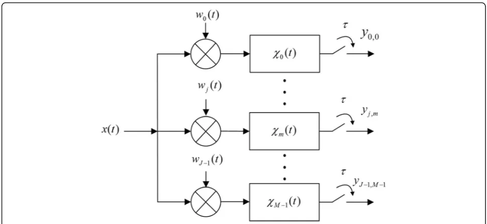
Equation (13) has an exceedingly simple form, as com-pared with that of the general settings discussed in [15]. Nonetheless, sm(t) is implemented with a filter.

First of all, construct function χ_mð Þ ¼t X

Evidently,χm(t) represents the unit impulse response of

the filter in the (j,m)th channel. What is notable is that

yjmis the integral result in timeτ=Wg(K−2N+ 1)/N.

Ac-cording to Eq. (13), τ=Wg(K2−K1−2N+ 1)/N= [T]≥T.

Consequently, if the sampling action occurs ints, it

sug-gests that the sample yj,m is acquired from the (j,m)th

channel. In addition, index m corresponds to n and the

total number of time domain transform functions equals the order of E-splines, namelyM=N. Figure 2 shows the transformation of Gabor sampling scheme withsm(t),

car-ried out by filters other than waveforms.

By inserting Eq. (6) into the expression, χm(t) can be

reduced to a simple form as χ_mð Þ ¼t e−αmN t=Wg_rect

t−T=2

ð Þ, which is an exponential function truncated by

a rectangle window supported in [0,T]. Then, the

Laplace transform ofχm(t) is expressed as

Xmð Þ ¼s

1−e−T sðþαmN=WgÞ sþαmN=Wg

ð15Þ

Besides the order of the E-splines and window width, the parameter vectorαis the adjustable variable that de-cides the filter characteristics. Each entry αmconsists of

real and imaginary parts. For the exponent item of Eq. (15), the real part was used to simplify the expression. Chooseαm=α0+imλ, wherem= 1, 2,…M. To fulfill the

convergence requirement of Laplace transform, it is ne-cessary that Re[s] >−α0. The optimal setting being α0=

Wg/WN, ifs=iω, forT≫Wand Wg≫W, it follows that e−T sþð αmN=WÞ¼_e−T Wg=W2_eiT mð λN=W−ωÞ→_{0 . Particularly, if}

Wg=W,α0 will have simpler form as α0= 1/N. In this

Xmð Þ ¼s sþαm1N=W. At the same time, for τ= [T]≥T, the

sample acquired int=ts, after passing the filter, does not

lose any signal information in interval [0,T].

3.3 Signal recovery and measurement matrix

As explained in Section 2.1, the relation between the samples yj,m and Gabor coefficients can be represented

with matrix Eq. (7). In this paper, Eq. (7) is reduced to

U=CZ, assuming in case that D=I. For every l, the

column vectors Z[l] of matrix Z have only S nonzero

entries out of K, which correspond to the pulse

loca-tions. Besides, all nonzero entries are in the same rows

of column vectors Z[l]. Matrix Z can be recovered by

solving MMV problem. In [22], it is suggested that, givenU∈ℝM×L

andC∈ℝM×KwithM<K, one can find:

Z′_{¼ arg min suppj Zjs:t:U¼CZ ð16Þ}

For this study, we focus mainly on the construction of

measurement matrixC. To bring out the concrete

meas-urement matrix cm,k, the first and foremost task is to fix

αm. For the above analysis, we have chosen αm=α0+

iλξ(m), with α0=Wg/NW, and here we just need to

decide λ. According to Eq. (10), cm;k ¼eαmkcm;0. If there is a component such as 2πiminλ, it is possible to con-struct a measurement matrix that has the same proper-ties as those of Fourier matrix. So, if we fixλ as λ= 2π/

K, thenαm¼_{N W}Wg þi2πξ_Kð Þm.

According to Section 3.2, and given that p,q∈{K1,

K1+ 1,…,K2},p+q=K−2N, we can compute cm,k as

follows:

cm;k ¼vm;q¼vm;ðK−2N−pÞ

¼

Z þ∞ −∞ e

−αmNt=Wgβ~ α ∼

−tN=WgþðK−2N−p−1Þ

dt

¼eαmðK−2N−pÞ

Zþ∞ −∞ e

−αmN t=Wgβ~ α ∼

−tN=Wg−1

dt

¼eαmq

Z þ∞ −∞ e

−αmNt=Wg_β~

−α∼ tN=Wg

dt

¼eαmk Ξð Þm Ξð Þm j j2;

ð17Þ

whereΞð Þ ¼m Wg

N YN

n¼1

1−eαnþαm αnþαm;

k∈fK1;K1þ1;…;K2g.

To avoid g(t) =β_α(tN/Wg) from being a

complex-valued function, we needαto be a vector with Im(αm) +

Im(αM−m) = 0, because βα(tN/Wg) is the convolution of

functions β_αm tN=Wg

and the convolution of β_αm

tN=Wg

and β_αM−m tN=Wg

generates a real value. So

for Imð Þ ¼αm i2πξ_Kð Þm ;m¼0;1;…;M−1, we can let

Imð Þ ¼αm

i2π

K ð2m−Mþ1Þ Mis even i2π

K

2m−Mþ1

2 Mis odd

8 > < >

: ð18Þ

Until now, we have deduced the representation of cm,k,

which is the (m,k)th entry of measurement C. And, we

also determine the parameter vector α, with the mth

entry expressed asαm¼_{W N}Wg þi2πξ_Kð Þm.

As there is still no effective and easy method to compute the RIC of such kind of matrices except ergodic calculating, we detect the RIP by comparing it with DFT matrix, which was proved to satisfy RIP for sparse signal reconstruction [23]. We need to explore the matrix coherenceθ. And for any matrixΦ, it is defined as [22]

Then by applying Gershgorin’s circle theorem, we can conclude that δS≤(S−1)θ(Φ). Furthermore, a (2S,δ

)-RIP matrix withδ2S< 1 necessarily has all subcollections

of 2Scolumns that are linearly independent, so, as [24], a normalized DFT matrix satisfies δ2S= (2S−1)θ(Φ).

Here, we use matrix coherence to judge the 2S-order

RIP of matrix C. Taking Eq. (17) into Eq. (19), we get

where θ(DFTQ) is a class of submatrices of Fourier

matricesDFT, which areK×Kmatrices with each entry as ðDFTÞ_m;k¼ 1ffiffiffi matrixCalso satisfies RIP and many other properties of

DFTQ. In [22], theorem 3.3 shows that for anyt> 1 and

anyK,S> 2, a random subsetQof average cardinality

M¼ðCtSlogKÞlogðCtSlogKÞlog2S ð21Þ

satisfies the RIP condition with probability of at least 1 −5e−ctand that theCwith possible indices denotes ab-solute constants. In any fixed probability of success such as 0.99, then Eq. (21) yields the best known bound on the number of Fourier measurementsM=O(Slog4K).

With Eq. (4), we are able to finish the signal recon-struction. The atoms of the dual Gabor frames

corre-sponding to the nonzero Gabor coefficients can

construct a Gabor subspace of the signal. Consequently, it can be said that a class of signals, constructed by the same kinds of pulses, belong to a union of Gabor

subspaces according to [5]. The recovery of Gabor coef-ficient matrixZis called subspace detection. So, for per-fectly reconstructing the original signal, the critical problem is how to construct the sampling scheme with appropriate relation betweenSandK.

In this study, we can solve the problem from the two entry points: the windows widthWgand the index set of

measurement matrixC. On the one hand, in a fixed time

duration,Kis determined by the time shifting parameter

a. With Wg increasing, K gets smaller. On the other

hand, Wg is intimately involved with sparsity S. If the

windows are wide enough, the sparsityS can be reduced

to half of that proposed in [15]. What is more, E-splines have a special property: the higher the orderN, the more the energy is centralized to a shorter time domain sup-port [18]. Then the essential window width gets short and the ratioM=S ¼N=Swas brought down.

4 Frame window width for sample number

In sampling scheme,Kis the dimension of vectors Z[l],

where there exists K ¼TþWg larger the ζ is increased, the smaller the K is. In [15], there existsWg=W, and soK′¼ _WTþ2

N−1. ForT≫

W, we can greatly reduceKby this way.

In another parameter, the sparsity is represented as S

¼ WgþW

see, wider window width also means smaller sparsityS. For more accurate analysis, we take a good property of E-splines into account: the higher the order N, the more the energy is centralized to a shorter time domain support [18]. Here, introducing the concept of “essential frame windows width,”we say thatφ(t) hasϵW-essential window

With the increase in the order N, the ϵW-essential

windows width WEgets shorter. Defining essential window

width factor η=WE/Wg, we can measure precisely how

of permissible η. Based on the foregoing assumption, the Then, the practical sparsity get smaller. As a result, to

ensure that C satisfy RIP, we need M¼O

ηζþ1

ζ NpNlog4ðT N=ζWÞ

. Note, in this study, M=N.

So, for perfect subspace detection, if there exists con-stantC'> 0, the following equation must be satisfied:

ηζþ1

by ζ. So, larger ζ means C has better orthogonality and better RIP. In addition, if we enlargeζ, Eq. (23) is easier to be satisfied. As the channel number of the sampling

scheme is decided by M, we can increaseN to acquire

more measured samples, which means better

recon-struction performance. As η and N are inversely

corre-lated in Eq. (23), sometimes we need not to worry that

Nis too large to prevent Eq. (23) from being satisfied. Next, we will analyze the effect of stretching the frame windows width on the signal reconstruction error. First, we offer a lemma here.

4.0.0.1 Lemma 1 For any Gabor window functions

g(t)∈S0, if there exists a constant 0 <ζ<∞, we have ation is as the following equation

Vg0g0ðτ;fÞ ¼ζ

According to the definition of Segal algebraic space, for any g(t)∈S0, kg tð Þk_S0<∞ is able to be satisfied under condition 0 <ζ<∞. So kg0ð Þt k_S0¼ζkg tð Þk_S0<∞

andg(t/ζ)∈S0. Prove up.

According to the lemma, if the windows are stretched

ζ times, the S0-norm is proportional to the stretching

factor. What is surely guaranteed is that the S0-norm

does not relate to the size of the grid in time and frequency plane and the redundancy. Consequently, we can propose the following theorem about the signal reconstruction error bound.

4.0.0.3 Theorem 2 Given thatx(t) is a finite duration sig-nal supported on the interval [0, T] withϵΩ-bandlimited

[−Ω/2,Ω/2], andGðg;a;bÞis a frame with each atomg(t) supported on [0, W] andϵB-bandlimited on [−B/2,B/2], of

which the dual atomγ(t)∈S0. For each atomg′(t) =g(t/ζ), with its dual atom γ′(t)∈S0, and ϵB> 0, there exist K1<

0 , K2> 0 and L0> 0, depending onγ(t) and the essential

bandwidths ofg(t), the following inequality is satisfied

x−X

The proof is rooted [15] with appropriate adjustments according to Lemma 1.

Theorem 2 shows that the reconstruction error is com-prised of two parts. The first part comes from Gabor series truncating and window cutting. For Gabor windowsg(t)

sup-ported on a quite short time interval, Cζ≈ 1þ_{ζW N}1

Withζincreasing,Cζdecreases evidently andC0is brought

down. Meanwhile, the higher the E-spline smoothness order

Nis, the smallerCζis, which results in the error reduction.

The second partζcomes from subspace detection error. As analyzed, largerζmeans thatChas better RIP, which can also decrease the error. So, we can reduce the signal reconstruc-tion error bound by enlarge window width.

The total number of Gabor coefficients is related to a somewhat larger interval [0,T'], whereT'=T+ 2ζW, with the required number of samples isK L≈T0N

ζWζWΩ

0 ¼T0Ω0 N. To decreaseKLfurther,b can be maintained constant at b¼1=W. Then L≈WΩ' and the size of matrix Z

be-comes K L≈T

0 Ω0N.

ζ. By this method, ifζis big enough,

the calculation load can be greatly reduced. Reducing Ga-bor coefficient numbers may enlarge the error bound, but we still can acquire acceptable error with suitable factorζ.

5 Noisy measurements

All the signals, hitherto considered for sampling, were noise-free or exactly multipulse. But when the signals to be measured are noisy, according to [15], the Gabor sampling scheme is robust to bounded noise in both the signal and the samples. Here, we will study the robust-ness of the sampling scheme proposed in this paper.

well approximated to a sparseZ, which consists of |Λ| rows ofZwith largestl2norm, and zeros, otherwise referred to as the best |Λ|-term approximation. If the indice setsΛis complete, |Λ| =S. Then, Eq. (7) can be written as

Y¼DUTþN′; withU¼CZþN ð25Þ

With Dhaving a full column rank, the relation to Eq.

(25) can be reduced to U=CZ+N, where N=D†N′. By utilizing CS algorithms,Z'can be resolved well even with noisy terms, and the following inequality, satisfying [25]:

Z−Z′

2≤C ′

1kZ−ZΛk2;1þC′2k kN 2 ð26Þ

where C '1and C '2are constants depending on the RIP

constant δ2S of C. Then, according to Theorem 2, we

can deduce the error bound as follows:

x−X k∈Λ

X

k¼−L0 L0

zk;lMb′lTa′kγ′

≤C0∥x∥2þC1kZ−ZΛk2;1þC2k kN 2

ð27Þ

where C0 is the same as that in Theorem 2, while C1 ¼ηζCζC′₁∥γ∥S0 andC2¼ηζCζC

′ 2∥γ∥S0.

Here, the third part of the error bound comes from the noise. As analyzed above, increasingζ and Nis also

beneficial to bring downCζand minimize the impact of

the noise. What is more, with increase in the smooth-nees orderNof the windows, the normsk kg _S0 andk kγ _S0 decrease rapidly, which is able to make the error bound

going down as well. To the contrary, if we increase N,

the RIP ofCmay get worse, andC'2, which is the

conver-gence factor for the noise, may be enlarged. Then, the noise suppression generated by the CS iteration will be weak. However, comparing the variation trends of the several factors following N,Cζand k kγ S0 play a leading

role on improving the sampling scheme robustness. IfN

rises, the redundancy of the Gabor frames would get higher. So, the analysis happens to coincide the conclu-sion in Eq. (26), which indicates that higher frames redundancy causes better robustness.

6 Simulation and discussion

We now present some numerical experiments to illustrate the reconstruction performance of short pulses with sub-Nyquist sampling, using the scheme proposed above.

The sampling scheme was tested on a range of

multi-pulse signals of duration T= 20ms, and the pulses

mak-ing up the signals were randomly chosen as a set of three different pulses: cosine, Gaussian, and B-spline of three orders. The number of pulses was varied between

Np= 1, 3, 5, the maximum pulse width being W= 0.5ms.

The locations of the pulses were also chosen at random. Monte Carlo method was used for simulations averaged

over 500 trials. Throughout the experiments, we chose

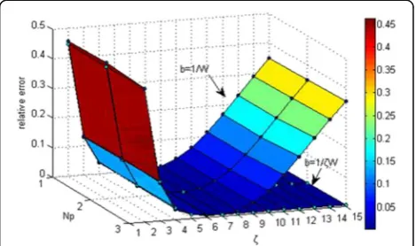
D=Iand measured the relative errorkx−^xk₂=k kx ₂. In the first experiment, we studied the effects of stretching Gabor frame windows width on the reconstruction error. The smoothness order of the E-spline windows was chosen

as a fixed number M=N= 100. The Gabor coefficients Z

was acquired by solving the MMV problem with SOMP. Figure 3 shows the relative error between the recon-structed signals and the original signals with the increase in window stretching factorζand the pulse numberNp. The

two curved surfaces represent respectively the error vari-ation trends under the conditions ofb= 1/Wandb= 1/ζW. It can be seen that whenb= 1/ζWandζ≥7, the signals can be reconstructed with minimum error, and the variation of

Np had little effect on the error. With increasing ζ, the

dimensionKofZsignificantly decreased, which means that the measurement matrix has correspondingly fewer col-umns, and can hence be recovered with higher accuracy. In this case, time samples satisfiedK≤716; also, Eq. (21) can be easily satisfied and even more pulses reconstructed. For reducing the size of Gabor coefficient matrixZ, we can also chooseb= 1/W. Whenζ≈7, the recovery error of the sig-nal will be approximately the same as that whenb= 1/ζW.

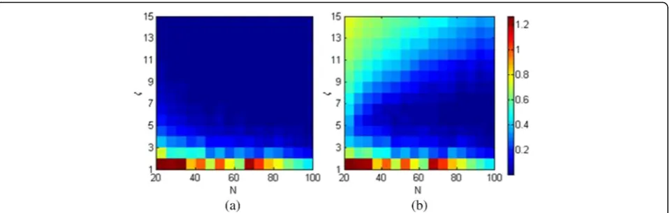
In the second experiment, we studied the effects of

E-spline smoothness order N on the relative

reconstruc-tion error under different stretching factor ζ. We chose

Np= 3 with no other signal parameters not changed. The

simulation was started withN= 25, addingNat uniform

intervalΔN= 5 untilN= 100, while the windows

stretch-ing factor ζ was raised from 2 to 15. The results are

shown by Fig. 4a, b. According to the figures, when N

was small, the error was generally large. In the case that

ϵW= 0.1 and N= 25, there existedη≈0.2, and the

mini-mum error was on the rowζ= 5. When Nwas not large

enough, the measurement matrix C was too flat to

re-cover Z perfectly. With increasing N, the optimal

stretching factor was raised to aboutζ= 7. WhenNwas

large enough, with appropriate ratio M/K and essential

Fig. 3Relative reconstruction error variation curve with the increasing of window stretching factorζand pulse numberNp

WE, the errors became quite small, enabling broadening

of the range of feasible window width.

In the third experiment, we verified the robustness of the proposed sampling scheme. In the simulation, with

Np= 3, Gaussian noise with noise/signal ratio (SNR) of

15 dB was injected into the channel. The smoothness orderNwas equivalent toM, increasing from 25 to 100. Figure 5 shows the SNR of output signals from the sam-pling schemes with redundancy μ¼1=N relating to this study, and with μ= 0.5,μ= 0.3,μ= 0.75 relating to [15]. It was seen that for the sampling scheme proposed, the

SNR increased with the raising ofN, improved by about

20 dB compared with that of the input signals. When the channel numbers were the same, it was generally much higher than that of the sampling scheme in [15], showing better performance on noise suppression.

Finally, we compared the reconstruction error of the sampling scheme proposed in this paper with that of a specific example in [15]. In Table 1, Schemes I and II

relate respectively to the sampling schemes proposed in this paper and that in [15]. As the scheme structure chan-ged significantly and, at the same time, the parametersM,

K, μ, and ζ could not remain the same, the comparison

was restricted to some typical cases with the same signal. Here, we choseNp= 3 and set other signal parameters as

they were before. Table 1 shows that, under appropriate parameter setting, the reconstruction performance of both schemes were similar. Therefore, the sampling scheme proposed here can be considered effective and feasible.

7 Conclusions

We introduced high order exponential reproducing win-dows into Gabor sampling scheme for sub-Nyquist sam-pling of short pulses, which notably simplified the filter’s structure of the sampling system and enabled it to be realized by RC filters. Subject to choosing an appropriate E-spline parameter vectorα, the Gabor windows could be a positive real function and it is possible to construct the measurement matrix as a weighted DFT matrix for Gabor coefficients recovery, which is proved to have good coher-ence. Meanwhile, we developed methods for good RIP by stretching windows and increasing E-spline smoothness orderN. With that, the ratiorof the row dimension and the column dimension of the measurement matrix could be improved. Also, the sampling system was proved to hold acceptable reconstruction error bound. Because the energy of the E-splines would concentrate to a narrower support with the increasing of N, the Gabor coefficient matrix holds lower sparsity and hence its recovery by using CS algorithms is more reliable. For reducing the coefficients of samples further, we compressed the dual Gabor frames and proved that the reconstruction of the original signals was still under a low error bound and that it benefited from the nice robustness caused by high frames redundancy. With high frames redundancy, the sampling scheme holds nice robustness.

Fig. 4Relative reconstruction error variation with increased E-spline smoothness orderNunder different stretching factors_ζ.ais in the case that

b=_ζ/Wwhenbis in the case thatb= 1/W

Acknowledgements

The experiments of this research were financially supported by the National Natural Science Foundation of China under Grant 61501493.

Authors’contributions

CW conceived and designed the study. PC carried out most of the analyses. CW, YW, and PC drafted the manuscript. CM, XS, and WL performed the experiments. All authors read and approved the final manuscript.

Competing interests

The authors declare that they have no competing interests.

Publisher’s Note

Springer Nature remains neutral with regard to jurisdictional claims in published maps and institutional affiliations.

Author details

1_{Shijiazhuang Mechanical Engineering College, Shijiazhuang 050003, China.}

2_{Tianjin University of Technology and Education, Tianjin 300222, China.}

3_{Mechanical Technology Institute, Shijiazhuang 050003, China.}

Received: 20 February 2017 Accepted: 4 April 2017

References

1. M Mishali, YC Eldar, Sub-nyquist sampling: bridging theory and practice. IEEE Signal Process. Mag.11, 98–124 (2011)

2. J Crols, S Michiel, J Steyaert, Low-if topologies for high-performance analog front ends of fully integrated receivers. IEEE Trans. Circuits Syst. II, Analog Digit. Signal Process.45(3), 269_–282 (1998)

3. Z Li, K Liu, Y Zhao et al., MaPIT: an enhanced pending interest table for NDN with mapping bloom filter. IEEE Commun. Lett.18(11), 1915–1918 (2014) 4. Z. Li, L. Song, and H Shi. Approaching the capacity of K-user MIMO

interference channel with interference counteration scheme.Ad Hoc Networks, 2016, 46(2), Accept for Publication. DOI:10.1016/j.adhoc.2016.02.009. 5. Z Li, Y Chen, H Shi, K Liu, NDN-GSM-R: a novel high-speed railway

communication system via Named Data Networking. EURASIP J Wirel. Commun. Net Work.48, 1_–5 (2016)

6. PL Dragotti, M Vetterli, T Blu, Sampling moments and reconstructing signals of finite rate of innovation: Shannon meets Strang–Fix. IEEE Trans. Signal Process.55(5), 1741–1757 (2007)

7. X. Liu, Z. Li, P. Yang, and Y. Dong. Information-centric mobile ad hoc networks and content routing: a survey.Ad Hoc Networks, 2016, http://dx. doi.org/10.1016/j.adhoc.2016.04.005.

8. R Tur, YC Eldar, Z Friedman, Innovation rate sampling of pulse streams with application to ultrasound imaging. IEEE Trans. Signal Process.59(4), 1827_– 1842 (2011)

9. Z Wu, X Xia, B Wang, Improving building energy efficiency by multiobjective neighborhood field optimization. Energ Buildings87, 45–56 (2015) 10. Z Wu, X Xia, Optimal switching renewable energy system for demand side

management. Sol. Energy114, 278–288 (2015)

11. Z Wu, TWS Chow, Binary neighbourhood field optimisation for unit commitment problems. IET Gener. Transm. Distrib.7(3), 298–308 (2013) 12. Z Wu, X Xia, Optimal motion planning for overhead cranes. IET Control

Theory Appl.8(17), 1833–1842 (2014)

13. G. Itzhak, E. Baransky, N. Wagner, et al. A hardware prototype for sub-nyquist radar sensing.//Systems, Communication and Coding (SCC), Proceedings of 2013 9th International ITG Conference on. VDE, 2013: 1–6. 14. T Michaeli, YC Eldar, Xampling at the rate of innovation. IEEE Trans. Signal

Process.60(3), 1121–1133 (2012)

15. E Matusiak, YC Eldar, Sub-nyquist sampling of short pulses. IEEE Trans. Signal Process.60(3), 1134–1148 (2012)

16. M Mishali, YC Eldar, From theory to practice: Sub-Nyquist sampling of sparse wideband analog signals. IEEE J. Sel. Topics Signal Process4(2), 375–391 (2010) 17. YM Lu, MN Do, A theory for sampling signal from a union of subspaces.

IEEE Trans. Signal Process.56(6), 2334–345 (2008)

18. M Unser, T Blu, Cardinal exponential splines: Part i-theory and filtering algorithms. IEEE Trans. Signal Process.53(4), 1425–1438 (2005)

19. H Olkkonen, JT Olkkonen, Measurement and reconstruction of impulse train by parallel exponential filters. IEEE Signal Process. Lett.15, 241–244 (2008) 20. H Olkkonen, JT Olkkonen, Sampling and reconstruction of transient signals

by parallel exponential filters. IEEE Trans. Circuits Syst. Express Briefs57(6), 426_–429 (2010)

21. T Kloos, J Stockler, M Ckler, Zak transforms and gabor frames of totally positive functions and exponential b-splines. J Approximation Thoery184, 209–237 (2013) 22. M. Rudelson, R. Vershynin. Sparse reconstruction by convex relaxation:

Fourier and gaussian measurements.Information Sciences and Systems, 2006 40th_{Annual Conference on, IEEE, 2006: 207–212.}

23. K. Grochenig. Foundations of time-frequency analysis. Boston, Springer. (2001)

24. HG Feichtinger, On a new segal algebra. Monatshefte fr Mathematik92(4), 269–289 (1981)

Submit your manuscript to a

journal and benefi t from:

7Convenient online submission 7Rigorous peer review

7Immediate publication on acceptance 7Open access: articles freely available online 7High visibility within the fi eld

7Retaining the copyright to your article

Submit your next manuscript at 7 springeropen.com Table 1Reconstruction errors of sampling scheme proposed in this paper and that in [15]

Parameters M =50 M= 75 M= 100

Scheme I b= 1/W,ζ= 7 0.0542 0.0168 0.0023

b= 1/W,ζ= 14 0.5525 0.3803 0.2912

b= 1/ζW,ζ= 7 0.0192 0.0108 0.0091

b= 1/ζW,ζ= 14 0.0093 0.0091 0.0090

Scheme II μ= 0.3 0.0053 0.0053 0.0053

μ= 0.5 0.0064 0.0064 0.0064

μ= 0.75 0.0113 0.0113 0.0113