Classes of sum of cisoids processes and their statistics for the modeling and simulation of mobile fading channels

R E S E A R C H

Open Access

Classes of sum-of-cisoids processes and their

statistics for the modeling and simulation of

mobile fading channels

Bjørn Olav Hogstad

, Carlos A Gutiérrez

, Matthias Pätzold

and Pedro M Crespo

Abstract

In this paper, we present a fundamental study on the stationarity and ergodicity of eight classes of sum-of-cisoids (SOC) processes for the modeling and simulation of frequency-nonselective mobile Rayleigh fading channels. The purpose of this study is to determine which classes of SOC models enable the design of channel simulators that accurately reproduce the channel’s statistical properties without demanding information on the time origin or the time-consuming computation of an ensemble average. We investigate the wide-sense stationarity, first-order stationarity of the envelope, mean ergodicity, and autocorrelation ergodicity of the underlying random processes characterizing the different classes of stochastic SOC simulators. The obtained results demonstrate that only the class of SOC models comprising cisoids with constant gains, constant frequencies, and random phases is defined by a set of stationary and ergodic random processes. The analysis presented here can easily be extended with respect to the modeling and simulation of frequency-selective single-input single-output (SISO) and multiple-input multiple-output channels. For the case of frequency-selective SISO channels, we investigate the stationarity and ergodicity in both time and frequency of 16 different classes of SOC simulation models. The findings presented in this paper can be used in the laboratory as guidelines to design efficient simulation platforms for the performance evaluation of modern mobile communication systems.

1 Introduction

Computer simulators have become fundamental tools for the design, test, and optimization of modern mobile communication systems [1]. They provide a powerful, affordable, and reproducible means to assess the system performance. An important component of any computer simulator employed for system analysis is the model cho-sen to simulate the channel. This is indeed a critical component as most of the problems affecting the per-formance of wireless communication systems, e.g., inter-symbol interference and cross modulation, are caused by the channel [2]. There exist several different approaches to the design of fading channel simulators, such as those described in [3-6]. While the underlying methodology may differ, the principal objective of all stochastic chan-nel simulators is the same: synthesizing a random process

*Correspondence: [email protected]

1CEIT and Tecnun, University of Navarra, Manuel de Lardizábal 15, San Sebastián 20018, Spain

Full list of author information is available at the end of the article

that can efficiently be realized on a software or hard-ware simulation platform under the constraint that its statistical properties resemble those of a nonrealizable reference channel model. A typical nonrealizable refer-ence channel model is, for example, the Rayleigh fading channel model under isotropic scattering conditions ([7], Sec. 2.1.2). A realizable random process constitutes the so-called channel simulation model ([8], Sec. 4.1).

Two often desirable properties of any stochastic simu-lation model for small-scale multipath radio channels are stationarity and ergodicity. These properties enable the channel simulator to accurately emulate the channel’s sta-tistical properties on the basis of a single simulation run (ergodicity) without requiring information on the time origin (stationarity). In the strict sense, a channel sim-ulator is stationary if all marginal and joint probability density functions (PDFs) of the underlying random pro-cess characterizing the simulation model are independent of a time-shift ([9], pp. 297–303). On the other hand,

a channel simulator is ergodic if the time averages of the simulation model are equal to the ensemble averages ([9], Sec. 13.1). These conditions are too stringent and can hardly be met in practice. However, the information about the channel’s statistics of order higher than 2 is rarely required to assess the performance of wireless commu-nication systems. Hence, for most practical purposes, it suffices if the channel simulator is wide-sense station-ary (WSS) and ergodic with respect to (w.r.t.) the mean value and the autocorrelation function (ACF). In [10,11], the advantages of ergodic channel simulators versus non-ergodic simulation models for the performance analysis w.r.t. the bit error probability have been demonstrated. More specifically, in [10], this observation has been done for noncoherent differential phase shift keying since the bit error probability depends on the ACF of the under-lying complex Gaussian process. If the channel simulator is nonergodic, time ACF of the simulation model does not fit well with ensemble ACF of the reference model. In this case, one needs to average over different realizations of the underlying stochastic process to increase the per-formance, which also drastically increases the complexity of the channel simulator. Indeed, an important aspect of the statistical characterization of a channel simulator con-sists in determining whether the simulation model is a WSS, a mean-ergodic (ME), or an autocorrelation-ergodic (AE) random process. For some applications, such as the evaluation of diversity systems ([7], Ch. 6), it is also very important to know whether the envelope of the simula-tion model is a first-order stasimula-tionary (FOS) process. An interesting study of the relation between the coherence interval and the spectral spread of a zero-mean WSS pro-cess and its application to mobile fading channels can be found in [12]. In addition, an investigation of the time interval within which the fading process is expected to ful-fill the stationarity assumption in real-world channels can be found in [13,14].

Among the variety of channel simulation models pro-posed in the literature, those based on Rice’s sum-of-sinusoids (SOS) principle [15,16] have widely been in use as a basis for the design of multipath radio channel simu-lators (e.g., see [17-21]). In the conventional SOS channel simulation approach, it is assumed that the inphase and quadrature (IQ) components of the channel’s complex envelope are statistically independent Gaussian processes. Under this consideration, the simulation of the channel’s IQ components is carried out by means of two uncor-related SOS processes having disjoint sets of parameters - gains, frequencies, phases, and number of sinusoids. This approach has been applied for over four decades to the simulation of a variety of mobile fading channels, ranging from simple single-input single-output (SISO) channels [18] to sophisticated input multiple-output (MIMO) channels [19]. It is important to notice

that the conventional SOS simulation approach suffers from a serious limitation, that is, it can only be used to simulate fading channels characterized by symmetrical Doppler power spectral densities (DPSDs), leaving aside the more realistic case of channels having asymmetrical DPSDs.aA solution to overcome this limitation provides a variation of the conventional SOS approach, where a finite sum of complex sinusoids (cisoids) is used to sim-ulate the channel’s complex envelope [22]. Basically, SOC models differ from conventional SOS models such that the IQ components of the former models are characterized by the same set of parameters [22]. This feature of SOC models enables the simulation of fading channels having symmetrical and asymmetrical DPSDs [23-26]. Another important feature of SOC models is that they have a clear physical meaning as they are related to the electromag-netic plane wave model [8,27]. This is in contrast to the conventional SOS model, which cannot be interpreted physically.

Despite the significant attention that SOC channel sim-ulation models have attracted, a comprehensive study on their stationary and ergodic properties is still lacking in the literature. To close this gap, we present in this paper a systematic analysis of the wide-sense stationarity, first-order stationarity of the envelope, mean ergodicity, and autocorrelation ergodicity of eight fundamental classes of SOC simulation models for frequency-nonselective SISO Rayleigh fading channels. This analysis can easily be extended with respect to the modeling and simula-tion of frequency-selective SISO and MIMO channels. For the case of frequency-selective SISO channels, we pro-vide in this paper a concise investigation of the stationarity and ergodicity in both time and frequency of 16 different classes of SOC simulation models. The presented results are intended to serve as guidelines for the design of effi-cient channel simulators for the performance evaluation of mobile communication systems.

The rest of the paper is organized as follows. In Section 2, we discuss the related work and highlight the novelty and importance of our paper. In Sections 3 and 4, we briefly review the reference model and the SOC model, respectively. In Section 5, we summarize the characteris-tics of stationary and ergodic processes. Section 6 intro-duces eight classes of SOC-based simulation models and investigates their stationary and ergodic properties. An extension to frequency-selective channels can be found in Section 7. A discussion of the obtained results and their applications to widely used parameter computation meth-ods can be found in Section 8. Finally, the conclusions are drawn in Section 9.

2 Related work

of conventional SOS simulators have thoroughly been analyzed in [28-30]. In these papers, the authors have analyzed the ME and AE properties of eight classes of deterministic and stochastic SOS simulation models for Rayleigh fading channels. They also investigated the wide-sense stationarity and the first-order stationarity of the IQ components of all eight classes of SOS channel simulators. It is shown in [28-30] that an SOS process is stationary and ergodic if and only if the sinusoids’ gains and Doppler frequencies are constant quantities and the phases are random variables. We notice, nonetheless, that the con-clusions drawn in these papers cannot be extrapolated to the case of SOC simulators. The reason is that the inves-tigations performed in [28-30] were carried out in the framework of the conventional SOS channel simulation approach, implying the condition that the IQ components of the channel simulation model are uncorrelated. This condition does not necessarily hold for SOC simulators, meaning that their IQ components are in general corre-lated [31]. It is precisely this particular feature that enables SOC models to simulate fading channels characterized not only by symmetrical DPSDs but also by asymmetri-cal ones. It is therefore necessary to revisit the analysis in [28-30] to shed light on the peculiar and important case of SOC channel simulators. The results presented in this paper will demonstrate that the distribution of the enve-lope and the autocorrelation properties of SOC models differ completely from what is known from conventional SOS models.

3 The reference model

A Rayleigh processζ(t)is defined as

ζ(t)= |μ₁(t)+jμ₂(t)|, (1)

whereμ₁(t)andμ₂(t)are zero-mean real Gaussian pro-cesses, each with variance σ₀2.b The process μ(t) = μ₁(t) + jμ₂(t) will be considered as a complex Gaus-sian process. In general, it is usually assumed thatμ₁(t) and μ₂(t) are uncorrelated, but in this paper, we have allowed them to be correlated. The correlation properties are described by the correlation matrix in ([32], eq. (17)). Here, a process X(t) is called a complex Gaussian pro-cess if each finite-dimensional vector [X(t1),. . .,X(tn)]T is a complex Gaussian vector. A complex random vec-tor is said to be Gaussian if its real and imaginary parts are jointly Gaussian [33]. Therein, it is shown that if the process μ(t) is proper (or circularly sym-metric), the density of the mentioned complex Gaussian vector is completely described by the ACF rμμ(τ )

E{μ∗(t)μ(t+τ )}.

According to the correlation model proposed by Clarke in [34] for two-dimensional scattering environments, the ACFrμμ(τ )ofμ(t)can be expressed as

rμμ(τ )=2σ02 2π

0

pα(α)ej2πfmaxcos(α)τdα. (2)

In the equation above,fmax is referred to as the maxi-mum Doppler frequency, andpα(α)denotes the density

function of the angle of arrival (AOA) of the incoming waves.

4 The SOC model

It is well known (see, e.g., [35-37]) that Rayleigh fading channel models, characterized by the complex Gaussian process μ(t), can be modeled and efficiently simulated using the SOC process

ˆ μ(t)=

N

n=1

cnej(2πfnt+θn), (3) where N denotes the number of cisoids, cn is called the gain, fn designates the Doppler frequency, and θn denominates the phase of thenth cisoid. The phasesθn are independent and identically distributed (i.i.d.) ran-dom variables, each following a uniform distribution over [ 0, 2π ). It is worth mentioning that the frequencies fn are related to the maximum Doppler frequencyfmaxand AOAsαnof the waves that reach the receiver antenna by means of the transformation

fn=fmaxcos(αn), n=1,. . .,N. (4)

These parameters have a strong influence on the tempo-ral correlation properties of SISO channels and also on the spatial and temporal correlation properties of MIMO channels. Furthermore, in [25], it is shown that the cisoids’ frequencies are directly related to the angles of departure of transmitted waves in mobile-to-mobile double Rayleigh fading channels.

Owing to the central limit theorem ([9], p. 278), the stochastic process μ(t)ˆ tends to the complex Gaussian processμ(t)asN→ ∞. From the results obtained in [22], it is straightforward to show that the obtained process μ(t)is proper. If the phasesθ_nare outcomes (realizations) of a random generator with a uniform distribution in the interval(0, 2π], then the stochastic processμ(t)ˆ results in the sample function

˜ μ(t)=

N

n=1

cnej(2πfnt+θn), (5)

which is completely deterministic.

In principle, each type of these parameters can be intro-duced as a random variable or constant. Hence, altogether, 23_{=8 classes of SOC models for Rayleigh fading channels} can be defined. If all parameters are constants, we obtain a completely deterministic process, denoted by ζ (t)˜ = | ˜μ(t)| = | ˜μ1(t)+jμ˜2(t)|. As opposed to this, at least one random variable is required to obtain a stochastic pro-cess, denoted byζ(t)ˆ = | ˆμ(t)| = | ˆμ₁(t)+jμˆ₂(t)|. For the performance evaluation of SOC simulation models with random/constant parameters, it is important to know the conditions for which the resulting stochastic process

ˆ

ζ(t) is stationary. Also, it is important to know under which conditions the stochastic processμ(t)ˆ results in an ergodic process. In the next section, we will review briefly the characteristics of stationary and ergodic processes.

5 Stationarity and ergodicity

A stochastic processζˆ(t) is calledstrict-sense stationary (SSS) ([9], p. 387) if its statistical properties are invariant to a shift of the origin. This means that the stochastic pro-cessesζˆ(t)andζ(tˆ +c) have the same statistics for any c∈R. It follows that themth-order density function must satisfy the equation

p_ζˆ(x1,. . .,xm;t1,. . .,tm)=pζˆ(x1,. . .,xm;

t1+c,. . .,tm+c), (6)

for all values oft1,. . .,tm, andc.

A stochastic processζ(t)ˆ is called FOS ([9], p. 392) if the density ofζˆ(t)satisfies

p_ζˆ(x;t)=p_ζˆ(x;t+c), (7)

for all values oftandc. This implies that the mean and the variance ofζ(t)ˆ are independent of time. If a stochastic process is SSS, then the process is also FOS. The inverse statement is not always true. For simplicity and brevity, we only investigate the FOS properties ofζˆ(t). A stochas-tic processζ(t)ˆ is calledasymptotically FOSif the density p_ζˆ(x;t+c)tends to a limit, which is independent ofcas c→ ∞([9], p. 392).

A stochastic processμ(t)ˆ is said to be WSS ([9], p. 388) ifμ(t)ˆ satisfies the following conditions:

1. The mean ofμ(t)ˆ is constant, i.e.,

E{ ˆμ(t)} =mμ_ˆ =const. (8)

2. The ACF ofμ(t)ˆ depends only on the time difference τ =t2−t1, i.e.,

rμ_ˆμˆ(t1,t2)=rμˆμˆ(τ ) (9)

where

rμ_ˆμˆ(t1,t2)=E{ ˆμ∗(t1)μ(tˆ 2)} (10)

rμ_ˆμˆ(τ )=E{ ˆμ∗(t)μ(tˆ +τ )}. (11)

Note that all SSS processes are WSS, but the converse need not be true. Following ([38], p. 422), we define a stochastic process μ(t)ˆ to be asymptotically WSS if its mean is constant and its ACFrμ_ˆμˆ(t1,t2)depends only on the time difference τ = t2 − t1 ast1 → ±∞ and/or

t2→ ±∞.

Furthermore, a stochastic process μ(t)ˆ is said to be mean ergodicif its ensemble averagemμ_ˆ equals the time

averagemμ_˜ofμ(t)˜ , i.e.,

mμ_ˆ =mμ˜ := lim

T→∞

1 2T

T

−T ˜

μ(t)dt. (12)

The stochastic processμ(t)ˆ is said to beautocorrelation ergodicif its ACFrμ_ˆμˆ(τ )equals the time ACFrμ˜μ˜(τ )of

˜ μ(t), i.e.,

rμ_ˆμˆ(τ )=rμ˜μ˜(τ ):= lim

T→∞

1 2T

T

−T ˜

μ∗(t)μ(t˜ +τ )dt.

(13)

6 Classification of channel simulators

In this section, eight classes of SOC simulation models for frequency-nonselective Rayleigh fading channels will be introduced, seven of which are stochastic simulation mod-els and one is completely deterministic. Before presenting a detailed analysis of the various classes of simulation models, some constraints are imposed on the three types of parameters. These constraints are as follows.

In cases, where the gainscn, frequenciesfn, and phases θ_n are random variables, it is reasonable to assume that their values are real and they are mutually indepen-dent. Also, it is assumed that the gains c1,c2,. . .,cN are i.i.d. random variables. The same is assumed for the sequences of random Doppler frequencies f₁,f₂,. . .,f_N and phasesθ1,θ2,. . .,θN.

Whenever the gains cn and frequencies fn are con-stant quantities, it is assumed that they are different from 0, such that cn = 0 and fn = 0 hold for all values of n = 1, 2,. . .,N. Further constraints might also be imposed on the SOC model. For example, it is required that all frequenciesfn are different. This latter condition is introduced to avoid correlations within the inphase (quadrature) component ofμ(t)˜ .

6.1 Class I channel simulators

Sinceμ(t)˜ is a deterministic process, its meanmμ˜ has to be determined using time averages instead of statistical averages. Using (5) and taking into account thatfn = 0, we obtainmμ_˜ = 0. Hence, we realize that the

determin-istic processμ(t)˜ of the simulation model has the same mean value as the stochastic processμ(t)of the reference model, i.e.,

mμ_˜ =mμ=0 . (14)

Similarly, the ACFrμ˜μ˜(τ )ofμ(t)˜ has to be determined

using time averages. By taking into account that all fre-quenciesfnare different, we can express the ACFrμ˜μ˜(τ )

ofμ(t)˜ in the following form

rμ_˜μ˜(τ )=

used in the next subsections.

6.2 Class II channel simulators

The channel simulators of Class II are defined by a set of stochastic processesζˆ(t) with constant gainscn, con-stant frequencies fn, and random phases θn, which are uniformly distributed in the interval (0, 2π]. Using our notation, the complex processμ(t)ˆ = ˆμ₁(t)+jμˆ₂(t)can approaches the Rayleigh density as N → ∞ andcn = σ0√2/N.

With reference to (17), we notice that the densityp_ζˆ(z) is independent of time. Furthermore, from (18) and (19), we can realize that conditions 1 and 2 (see (8) and (9)) are fulfilled, respectively. Hence, the stochastic process

ˆ

ζ(t) is FOS, and the stochastic process μ(t)ˆ is WSS. A specific realization of the random phasesθ_nconverts the

stochastic processμ(t)ˆ into a deterministic process (sam-ple function)μ(t)˜ . This allows us to interpret Class I as a subset of Class II. The stochastic process μ(t)ˆ is ME since the identitymμ_ˆ = mμ˜ holds. Also, the stochastic

processμ(t)ˆ is AE. This statement follows from a com-parison of (19) and (15), which reveals that the criterion rμ_ˆμˆ(τ )=rμ˜μ˜(τ )is fulfilled.

6.3 Class III channel simulators

The channel simulators of Class III are defined by a set of stochastic processesζˆ(t)with constant gainscn, random frequenciesf_n, and constant phasesθ_n. Hence, the com-plex processμ(t)ˆ = ˆμ₁(t)+jμˆ₂(t)has the following form

To obtain the densityp_ζˆ(z;t) of the stochastic process ˆ

ζ(t), we continue as follows. In the first step, we consider a single complex cisoid at a fixed time instantt=t0. Thus,

ˆ

μ_n(t0)=cnej(2πfnt0+θn) (21)

describes a complex random variable. From [29], in the limit |t0| → ∞, the density pμˆ1,n(x1) of μˆ1,n(t0) =

Now, by following the same procedure as described in [22], we can conclude that the densityp_ζˆ(z;±∞)is given by (17). Iftis finite, we must replace the expression in (22) by ([29], Eq. (32)). In this case, it turns out that the density p_ζˆ(z;t)depends on timetso that the stochastic process

ˆ

ζ(t) is not FOS. Thus, we can conclude that a Class III channel simulator is an asymptotically FOS process.

In the following, we assume that the random frequen-ciesf_nare given by

f_n=fmaxcos(αn) (23)

where the AOAs α_n, n = 1,. . .,N, are i.i.d. random variables, each having a density pα(α) identical to that

characterizing the reference model’s AOA statistics. The mean mμ_ˆ(t) of the stochastic process μ(t)ˆ is

obtained by computing the statistical average of (20) with respect to the random characteristics of the frequencies f_n. Hence, we can write

whererμμ(t)is the ACF of the reference model described

in (2). From (24), we see that the meanmμ_ˆ(t)changes

N

n=1

cnejθn=0 . (25)

The condition above can easily be fulfilled if the num-ber of cisoidsNis even; the gainscnare constants given by cn = σ0√2/N, and θn = −θn+N/2 = π/2 for n = since it is given as

rμˆμˆ(t1,t2)= impose the following boundary condition on the gains and phases

In case that the above boundary condition is fulfilled and the gainscnare equal tocn =σ0√2/N, we easily see that the ACFrμ_ˆμˆ(τ )of the stochastic simulation model

is identical to the ACFrμμ(τ )of the reference model.

In Appendix 1, it is shown that conditions (25) and (27) cannot be simultaneously satisfied. However, if we lett1 → ±∞and/ort2 → ±∞, then the ACFsr∗μμ(t1) and/orrμμ(t2)tend to zero, and hence the ACFrμˆμˆ(t1,t2) depends only on the time differenceτ = t2−t1. In this case, together with the condition given in (25), we can conclude that the stochastic process μ(t)ˆ is an asymp-totically WSS process. Furthermore, if t → ±∞, then

ˆ

μ(t)tends to an asymptotically FOS process. The stochas-tic process μ(t)ˆ is ME since the condition mμ_ˆ = mμ˜

is fulfilled. However, the stochastic processes μ(t)ˆ of Class III channel simulators are always non-AE because the inequalityrμ_ˆμˆ(τ )=rμ˜μ˜(τ )holds.

6.4 Class IV channel simulators

The channel simulators of Class IV are defined by a set of stochastic processesζˆ(t) with constant gainscn, ran-dom frequencies f_n, and random phases θ_n, which are uniformly distributed in the interval(0, 2π]. In this case, the complex processμ(t)ˆ = ˆμ₁(t)+jμˆ₂(t)is given by as the random frequenciesf_nhave no effect on the density

p_ζˆ(z)in (17). The meanmμ_ˆ(t)is given by (18). If the gains

cnare equal tocn = σ0√2/Nand the frequenciesfnare given by (23), then it is straightforward to show that the ACFrμ_ˆμˆ(τ )of the stochastic simulation model is identical

to the ACFrμμ(τ )of the reference model, i.e.,rμˆμˆ(τ ) =

rμμ(τ ). The stochastic processesμ(t)ˆ of Class IV

chan-nel simulators are non-AE since the inequalityrμ_ˆμˆ(τ ) =

rμ_˜μ˜(τ )holds.

6.5 Class V channel simulators

A Class V channel simulator is determined by a stochastic processζ(t)ˆ with random gainscn, constant frequencies fn, and constant phases θn. Thus, the complex process

ˆ function of time. Hence, the stochastic processζ(t)ˆ is not an FOS process.

In the following, we will impose on the stochastic chan-nel simulator that the i.i.d. random variablescnhave zero mean and variance σ_c2, i.e.,mc = E{cn} = 0 andσc2 =

By taking into account that the gainscn have zero mean, i.e.,mc=0, we obtain

6.6 Class VI channel simulators

The channel simulators of Class VI comprise a set of stochastic processesζ(t)ˆ with random gainscn, constant frequenciesfn, and random phasesθn. In this case, the complex processμ(t)ˆ = ˆμ₁(t)+jμˆ₂(t)is of type Class VI channel simulators, we make use of the condi-tional density p_ζˆ(z|cn = cn) of Class II channel simu-lators. The densityp_ζˆ(z) of Class VI channel simulators can then be obtained by averaging the conditional den-sity p_ζˆ(z|cn = cn) over the distribution pc(y) of the N pendent of time. Hence, the stochastic processζ(t)ˆ is FOS. The meanmμ_ˆ(t)of the stochastic processμ(t)ˆ is still given

by (18) since the behavior of the random gainscnhas no effect on the mean in (18).

The ACFrμ_ˆμˆ(τ )of the stochastic processμ(t)ˆ can be

Without imposing any specific distribution on the random gainscn, we can conclude that the stochastic processμ(t)ˆ is non-AE since the inequalityrμ_ˆμˆ(τ )=rμ˜μ˜(τ )holds.

6.7 Class VII channel simulators

This class of channel simulators involves all stochastic processes ζ(t)ˆ = | ˆμ(t)| with random gainscn, random frequenciesf_n, and constant phasesθn, i.e.,

ˆ

To obtain the density p_ζˆ(z) of the stochastic process ˆ

ζ(t), we consider first the caset→ ±∞. The densityp_ζˆ(z) can be considered as the conditional densityp_ζˆ(z|cn=cn) obtained for Class III channel simulators. By following the same procedure described in SubSection 6.6, we can con-clude that the densityp_ζˆ(z)is given by (34). Iftis finite, we have to repeat the procedure described in SubSection 6.6 using ([29], Eq. (32)) instead of (22). In this case, it turns

out that the densityp_ζˆ(z;t)is a function oft. Hence, the stochastic processesζ(t)ˆ of Class VII channel simulators are asymptotically FOS processes.

The mean mμ_ˆ(t)of this class of channel simulators is

given by

It follows from (37) that the mean value is time indepen-dent if any of the boundary conditionsmc=0,t→ ±∞, or (25) are fulfilled.

Let us assume that the random frequenciesf_nare given by (23). Then, the ACFrμˆμˆ(t1,t2) of the stochastic pro-cessμ(t)ˆ is obtained by computing the statistical average of (31) with respect to the random characteristics of the frequenciesf_n. Thus, we obtain

rμ_ˆμˆ(t1,t2)=

From the equation above, it follows that the ACF rμ_ˆμˆ(t1,t2)depends only on the time differenceτ =t2−t1 if we impose on this class of channel simulators any of the boundary conditions mc = 0 or (27). In addition, similar to the explanations given in SubSection 6.3, we can conclude that the ACF rμ_ˆμˆ(t1,t2) depends only on the time difference τ = t2 − t1 if t1 → ±∞ and/or

t2→ ±∞. Furthermore, remember from SubSection 6.3 that the conditions (25) and (27) cannot be fulfilled simul-taneously. If any of the boundary conditionsmc = 0 or (27) is fulfilled and ifσ_c2= 2σ₀2/N−m_c2, thenrμˆμˆ(t1,t2) in (38) reduces to

rμ_ˆμˆ(t1,t2)=rμˆμˆ(τ )=rμμ(τ ), (39)

which states that the channel simulators of Class VII and the reference model have identical correlation properties. However, the stochastic processμ(t)ˆ is non-AE since the inequalityrμ_ˆiμˆi(τ )=rμ˜iμ˜i(τ )holds.

6.8 Class VIII channel simulators

The channel simulators of Class VIII are defined by a set of stochastic processesζ(t)ˆ = | ˆμ(t)|with random gains by (34) because the random behavior of the frequencies f_nhas no influence onp_ζˆ(z). Hence, a Class VIII channel simulator is FOS.

ˆ

μ(t) is constant and equal to zero, i.e., mμ_ˆ = 0. From

(38), we can easily obtain the ACFrμˆμˆ(τ )for this class

of channel simulators by taking into account the random characteristics of the phasesθn, i.e.,

rμ_ˆμˆ(τ )=

N(σ_c2+m2_c)

2σ₀2 rμμ(τ ). (41)

Hence,rμ_ˆμˆ(τ ) = rμμ(τ )holds ifσ_c2 = 2σ₀2/N−m2_c.

Note that in contrast to Class VII channel simulators, the ACF of Class VIII channel simulators only depends on the time differenceτ = t2−t1even ifmc=0. However, the channel simulators of Class VIII prove to be non-AE since the inequalityrμ_ˆiμˆi(τ )=rμ˜iμ˜i(τ )holds.

7 Extension with respect to frequency selectivity In this section, we extend our fundamental study on the stationarity and ergodicity of SOC simulation models for frequency-nonselective channels to SOC simulation mod-els for frequency-selective channmod-els. The time-variant impulse response, denoted by h(τ˜ ,t), of deterministic SOC simulation models for frequency-selective channels can be expressed in the equivalent complex baseband by the following ([8], Eq. (3.9))

˜

whereτ_nis the propagation delay of thenth path. For rea-sons of causality, we impose thatτ_n ≥0 forn=1,. . .,N. Furthermore, the time-variant channel transfer function, denoted by H(f˜ ,t), is obtained by taking the Fourier transform ofh(τ˜ ,t)with respect toτ , i.e.,

The time-variant channel transfer function H(f˜ ,t) depends on four types of parameters, namely the gains cn, the frequenciesfn, the phasesθn, and the propagation delaysτ_n. Each of these parameters can be defined either as a random variable or as a constant quantity. Hence, altogether, 24_{= 16 classes of SOC models for} frequency-selective Rayleigh fading channels can now be defined. The ACF, denoted byr˜HH(f ,f +ν;t,t+τ ), of the time-variant channel transfer functionH(f˜ ,t), defined by ([8], Eq. (7.144))

is called the time-frequency correlation function. After substituting (43) in (44) and taking into account that all frequenciesfnare supposed to be different, we obtain

˜

From (45), we can easily express the frequency correlation functionr˜HH(ν)and the time correlation functionr˜HH(τ )

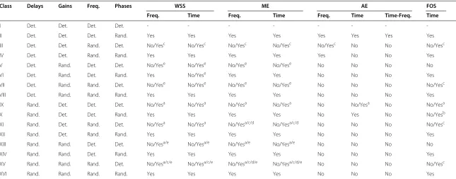
respectively. We notice that the two expressions in (46) and (47) are dual to each other. The duality allows us to deduce the properties of the frequency correlation function˜rHH(ν)directly from the properties of the time correlation function˜rHH(τ )if we replace the determinis-tic (random) frequenciesfn(fn)by deterministic (random) propagation delaysτ_n(τ_n). After a straightforward inves-tigation of the wide-sense stationarity, mean ergodicity, autocorrelation ergodicity with respect to both frequency and time, and the first-order stationarity of the envelope of the underlying random processes characterizing the 16 different classes of frequency-selective SOC simulators, we obtain the results presented in Table 1. For reasons of brevity, we have omitted the detailed calculations leading to the results in Table 1.

8 Discussion and applications to the design of channel simulators

al.

E

URASIP

Journal

o

n

W

ireless

C

ommunications

and

N

etworking

2013,

2013

:125

Page

9

o

f

1

5

Table 1 Classes of frequency-selective SOC models and their stationary and ergodic properties

Class Delays Gains Freq. Phases WSS ME AE FOS

Freq. Time Freq. Time Freq. Time Time-Freq. Time

I Det. Det. Det. Det. - - -

-II Det. Det. Det. Rand. Yes Yes Yes Yes Yes Yes Yes Yes

III Det. Det. Rand. Det. No/Yesc No/Yesc No/Yesc No/Yesc No/Yesc No No No/Yesc

IV Det. Det. Rand. Rand. Yes Yes Yes Yes Yes No No Yes

V Det. Rand. Det. Det. No/Yese _No/Yese _No/Yese _No/Yese _{No No No No}

VI Det. Rand. Det. Rand. Yes No/Yese _{Yes Yes No No No Yes}

VII Det. Rand. Rand. Det. No/Yese _No/Yese _No/Yese _No/Yese _{No No No No/Yes}c

VIII Det. Rand. Rand. Rand. Yes Yes Yes Yes No No No Yes

IX Rand. Det. Det. Det. No/Yesa No/Yesa No/Yesa No/Yesa No No/Yesa No No/Yesa

X Rand. Det. Det. Rand. Yes Yes Yes Yes No Yes No No/Yesb

XI Rand. Det. Rand. Det. No/Yesa No/Yesa No/Yesa/c/d No/Yesa/c/d No No No No/Yesc

XII Rand. Det. Rand. Rand. Yes Yes Yes Yes No No No Yes

XIII Rand. Rand. Det. Det. No/Yesa/e No/Yesa/e No/Yesa/e No/Yesa/e No No No No

XIV Rand. Rand. Det. Rand. Yes Yes Yes Yes No No No Yes

XV Rand. Rand. Rand. Det. No/Yesa/c/e No/Yesa/c/e No/Yesa/c/d/e No/Yesa/c/d/e No No No No/Yesc

XVI Rand. Rand. Rand. Rand. Yes Yes Yes Yes No No No Yes

Freq., frequency; WSS, wide-sense stationary; ME, mean-ergodic; AE, autocorrelation ergodic; FOS, first-order stationary; Rand., random; Det., deterministic.a_{Only in the limitf → ±∞;}b_{Only in the limitf →0;}c_{Only in the}

limitt→ ±∞;d_{If the boundary condition}N

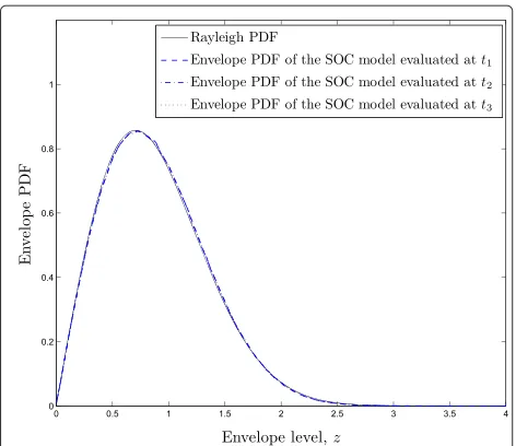
FOS envelope. However, from the results presented in Section 7, we can conclude that the channel simulators developed by Schulze and Höher are not AE. This is graphically demonstrated in Figure 1, where we present a comparison between the ensemble ACF and the time ACF of the channel simulator proposed in [41] withN = 20 cisoids, σ₀2 = 1, andfmax = 100 Hz. Here, we assume that all the delays are equal to zero so we only consider frequency-nonselective channels. The curves depicted in this figure were obtained by considering the simulation of a mobile fading channel satisfying the isotropic scatter-ing condition. Unless stated otherwise, the same setup is considered for all simulation examples presented through-out this section. Figure 2 provides a comparison between the Rayleigh distribution and the envelope PDF of the SOC model in [41] evaluated at three randomly chosen observation time instantst1,t2, andt3. The graphs shown in Figure 2 demonstrate that the envelope of the SOC simulation model is an FOS process.

A different type of frequency-nonselective SOC model was introduced in [42] by Crespo and Jimenez to simulate WSSUS channels by applying a harmonic decomposition technique to compute the model parameters. The SOC simulator considered in that paper is defined by cisoids with constant (null) phases, constant frequencies, and random gains, where it is assumed that the cisoids’ gains have zero mean. The underlying simulation model is thus a Class V SOC process that satisfies the conditions for wide-sense stationarity and mean ergodicity. However, it does not fulfill the conditions for autocorrelation ergod-icity, and its envelope is not an FOS process. This is numerically demonstrated in Figures 3 and 4, where we have again considered the simulation of a mobile fading

Figure 1Ensemble and time ACFs of the Class III SOC channel simulator proposed in [39,41].

Figure 2Comparison between Rayleigh distribution and envelope PDF of the Class III SOC channel simulator proposed in [39,41].

channel under isotropic scattering conditions. The graphs presented in Figures 3 and 4 where obtained by setting the relevant parameterspandT of the method in [42] equal top = 0.05 andT = 20/fmax. For this simulation setup, the resulting number of cisoids in SOC model equalsN= 281. It should be mentioned that the computational com-plexity by applying a harmonic decomposition technique has been addressed in [43].

The authors of [44] proposed a deterministic simula-tor for direction-selective and frequency-selective mobile radio channels. The generated waveforms of the simulator

Figure 4Comparison between Rayleigh distribution and envelope PDF of the Class V SOC channel simulator proposed in [42].

can be interpreted as sample functions of the frequency-selective Class II SOC model having cisoids with ran-dom phases uniformly distributed over the interval (0, 2π]. A channel simulator of frequency-nonselective or frequency-selective Class II SOC model corresponds in practice to scenarios where the scatterers around the receiver introduce constant gains and random phases. Furthermore, in these scenarios, the AOAs of the incom-ing waves are considered as constants due to the constant Doppler frequencies. Frequency-selective SOC channel models of Class II play an important role in the design of measurement-based channel simulators [45,46]. The correlation functions of such channel simulators match the correlation functions of measured channels accu-rately over a wide range determined by the length of the measured data. This can be achieved using the iter-ative nonlinear least square approximation method [47], which results in constant delays, constant gains, and constant Doppler frequencies, corresponding to constant AOAs. As the phases have no influence on the corre-lation functions, they are usually assumed to be i.i.d. uniform random variables. The assumption of constant AOAs has been applied in the well-known one-ring scat-tering model as demonstrated in [48,49]. Therein, the statistical properties of the presented channel simulator can be fitted nearly perfectly to the corresponding sta-tistical properties of a reference model where the AOAs are continuous random variables with a given distribu-tion. Hence, by considering constant AOAs in the channel simulator, we are able to simulate a large number of dif-ferent propagation environments. From Sections 6 and 7, it follows that a random process characterizing a channel

simulator as a nonselective or frequency-selective Class II SOC model is WSS, ME, and AE [49]. In addition, the envelope of the generated complex wave-forms proves to be an FOS process. These observations are supported by the simulation results shown in Figures 5 and 6, where we present plots of the ensemble ACF, time ACF, and envelope PDF of the frequency-selective Class II SOC simulation model proposed in [44]. For the simulation results presented in Figures 5 and 6, we have again considered the case that all the delays are equal to zero.

Building upon the simulation models introduced in [39,41,42,44], other researchers have developed new parameter computation methods to increase the simula-tor’s accuracy and to reduce the simulation setup time. The characteristics of some noteworthy parameter com-putation methods are summarized in Table 2. We refer the interested reader to [8,26,36] for a detailed discussion on the performance of the parameter computation methods listed in Table 2.

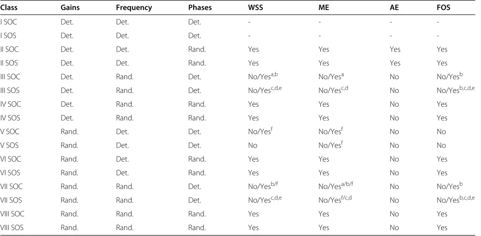
Before closing this section, it is worth noticing that the stationary and ergodic properties of the eight classes of frequency-nonselective stochastic SOC and SOS mod-els bear strong similarities as one may observe from the results presented in this paper and those obtained in [28-30]. A summary of the results obtained in this paper and those presented in [28-30] is given in Table 3.

This table shows that there exist some subtle but impor-tant differences between SOC and SOS models. For example, we have demonstrated that the SOC models of Class III are strictly non-WSS processes, whereas the SOS

Figure 6Comparison between Rayleigh distribution and envelope PDF of the Class II SOC channel simulator proposed in [44].

models of Class III are WSS if some boundary conditions are fulfilled [29]. On the other hand, we have shown that the SOC models of Class V are WSS if the random gains of the cisoids have zero mean. In contrast, it is demon-strated in [30] that the SOS models of Class V are strictly non-WSS.

9 Conclusions

In this paper, we provided a comprehensive analysis of the stationary and ergodic properties of eight classes of deterministic and stochastic SOC simulation models for frequency-nonselective mobile Rayleigh fading channels. We conclusively demonstrated that only the class defined by SOC models having cisoids with constant gains, con-stant Doppler frequencies, and random phases enables the design of channel simulators possessing the desired WSS, ME, AE, and FOS properties. In practice, this cor-responds to scenarios where the scatterers around the

receiver introduce constant gains and random phases. Furthermore, in these scenarios, the AOAs of the incom-ing waves are considered as constants due to the constant Doppler frequencies. Also, such a channel simulator can have nearly the same statistical properties as a given ref-erence model where the AOAs are random variables with a given distribution. Furthermore, such a channel sim-ulator that is extended to frequency-selective channels plays an important role in the design of measurement-based channel simulators. Hence, the channel simulator can be applied to a wide range of different propagation environments. The main focus of our work is on provid-ing a solid and comprehensive framework that researchers can use to determine if a particular class of SOC mod-els is well suited for the simulation of a given type of channel. For example, if one aims to simulate a fading channel having an FOS envelope, then it follows from the results presented in this paper that the SOC mod-els of Class V are not a suitable option. A comparison with the results obtained in other papers for the stationary and ergodic properties of conventional SOS models shows that the stochastic SOC models and the SOS models have similar properties. However, there exist some important differences between the properties of both types of sim-ulation models. Furthermore, we investigated the WSS, ME, AE, and FOS properties of SOC processes for the modeling and simulation of frequency-selective channels. Our investigations are of fundamental importance for the modeling and simulation of both SISO and MIMO channels.

The ergodic properties of Class II simulators for both frequency-nonselective and frequency-selective channels hold, provided that the lengths of the generated wave-forms (sample functions) are infinite. Unfortunately, this condition cannot be fulfilled in practice. In order to deter-mine whether the aforementioned properties hold under realistic simulation conditions, it is necessary to revisit the analysis presented in this paper by considering waveforms of finite length. We leave this important open problem for future research.

Table 2 Overview of parameter computation methods for SOC models and statistical properties of resulting channel simulators

Parameter computational method Class WSS ME AE FOSa

Monte Carlo method [39,41] IV Yes Yes No Yes

Harmonic decomposition technique [42] V Yes Yes No No

Lp-norm method [44] II Yes Yes Yes Yes

Method by Zheng [24] IV Yes Yes No Yes

Extended method of exact Doppler spread [25] II Yes Yes Yes Yes

Generalized method of equal areas [26] II Yes Yes Yes Yes

Riemann sum method [36] II Yes Yes Yes Yes

Table 3 Classes of SOC and SOS models and their stationary and ergodic properties

Class Gains Frequency Phases WSS ME AE FOS

I SOC Det. Det. Det. - - -

-I SOS Det. Det. Det. - - -

-II SOC Det. Det. Rand. Yes Yes Yes Yes

II SOS Det. Det. Rand. Yes Yes Yes Yes

III SOC Det. Rand. Det. No/Yesa,b No/Yesa No No/Yesb

III SOS Det. Rand. Det. No/Yesc,d,e No/Yesc,d No No/Yesb,c,d,e

IV SOC Det. Rand. Rand. Yes Yes No Yes

IV SOS Det. Rand. Rand. Yes Yes No Yes

V SOC Rand. Det. Det. No/Yesf No/Yesf No No

V SOS Rand. Det. Det. No No/Yesf No No

VI SOC Rand. Det. Rand. Yes Yes No Yes

VI SOS Rand. Det. Rand. Yes Yes No Yes

VII SOC Rand. Rand. Det. No/Yesb/f No/Yesa/b/f No No/Yesb

VII SOS Rand. Rand. Det. No/Yesc,d,e _No/Yesf/c,d _{No No/Yes}b,c,d,e

VIII SOC Rand. Rand. Rand. Yes Yes No Yes

VIII SOS Rand. Rand. Rand. Yes Yes No Yes

WSS, wide-sense stationary; ME, mean-ergodic; AE, autocorrelation ergodic; FOS, first-order stationary; Rand., random; Det., deterministic.a_{If the boundary condition}

N

n=1cnexp{jθn} =0is satisfied;bOnly in the limitt→ ±∞;cIf the density of the random Doppler frequencies is an even function;dIf the boundary condition Ni

n=1cos(θi,n)=0is satisfied;eIf the boundary conditionNni=1cos(2θi,n)=0is satisfied;fIf the mean value of the random gains is equal to zero.

Appendix 1

In this appendix, we will prove that the boundary condi-tions in (25) and (27) cannot be satisfied simultaneously. To that end, we observe that the equation in (27) is equivalent to

N

n=1

cnejθn N

m=1

cme−jθm− N

n=1

c2_n=0 . (48)

Now, if (25) holds, then we have from (48) that

N

n=1

c2_n=0 . (49)

The equation above poses a condition that cannot be sat-isfied because the cisoids’ gainscnare different from zero,

and therefore, N n=1

c2_n>0. This concludes the proof.

Appendix 2

In the following, we derive the density function of a stochastic process ζ(t)ˆ with random gains cn, constant frequenciesfn, and constant phasesθn. The starting point for the derivation of the density of the stochastic process

ˆ

ζ(t)= | ˆμ(t)|is a single complex cisoid of the form

ˆ

μ_n(t)=cnej(2πfnt+θn). (50)

For fixed values of t = t0, μˆ1,n(t0) = Re{ ˆμn(t)} = cncos(2πfnt0 + θn) and μˆ2,n(t0) = Im{ ˆμn(t)} =

cnsin(2πfnt0+θn)represent two dependent random vari-ables. From ([9], Eq. (5-18)), the density pμ_ˆ1,n(x1;t0) of

ˆ

μ_1,n(t0)can be expressed as

pμ_ˆ1,n(x1;t0)=

pc(x1/cos(2πfnt0+θn)) |cos(2πfnt0+θn)|

, (51)

wherepc(·)denotes the common density of the gainscn. Using ([50], Eq. (3.15)), the joint densitypμ_ˆ1,nμˆ2,n(x1,x2;t0)

of the dependent random variablesμˆ_1,n(t0) andμˆ2,n(t0) can be obtained as

pμ_ˆ1,nμˆ2,n(x1,x2;t0)=pμˆ1,n(x1;t0)δ(x2−g(x1;t0)) (52)

whereg(x1;t0) = x1tan(2πfnt0+θn). The joint charac-teristic function μ_ˆ1,nμˆ2,n(ν1,ν2;t0) of the random

vari-ables μˆ_1,n(t0) and μˆ2,n(t0) is defined by the Fourier transformation

_{μˆ1,nμˆ2,n}(ν₁,ν₂;t0)= ∞

−∞ ∞

−∞

pμ_ˆ1,nμˆ2,n

(x1,x2;t0)ej2π(ν1x1+ν2x2)dx1dx2.

(53)

After substituting (52) in (53) and carrying out some algebraic computations, we find

_{μˆ1,nμˆ2,n}(ν₁,ν₂;t0)= ∞

−∞

pc(x1)ej2π ν1x1cos(2πfnt0+θn)

ej2π ν2x1sin(2πfnt0+θn)_dx

1.

Since we have assumed that the gains cn are i.i.d. ran-dom variables, it follows that the quantities μ_n(t0) are also i.i.d. random variables. Hence, the joint character-istic function μ_ˆ1μˆ2(ν1,ν2;t0) of μˆ1(t0) and μˆ2(t0) can

be expressed as the product of the joint characteristic functionsμ_ˆ1,nμˆ2,n(ν1,ν2;t0)ofμˆ1,n(t0)andμˆ2,n(t0), i.e.,

From this and the two-dimensional inversion formula for Fourier transforms, it follows that the joint den-sitypμ_ˆ1μˆ2(x1,x2;t0)of the statistically dependent random

If we now transform the Cartesian coordinates(x1,x2) into polar coordinates(z,ϕ)by means ofx1=zcosϕand the envelopeζ(tˆ 0)can be obtained from the joint density

p_ζˆϑˆ(z,θ;t0)by integrating overϕ. By following this pro-cedure, using ([51], Eq. (3.937.2)) and transforming the Cartesian coordinates(ν1,ν2)into polar coordinates(r,θ ),

a_{We notice, nonetheless, that the conventional SOS}

simulation approach can be applied to the simulation of fading channels with asymmetrical DPSDs if the conventional approach is used in connection with the Hilbert transform ([8], Sec. 6.1.4).

b_{For clarity, we will use bold letters to indicate}

stochastic processes as well as random variables, and normal letters are used for deterministic processes (sample functions) and realizations (outcomes) of random variables.

Competing interests

The authors declare that they have no competing interests.

Acknowledgements

This paper was presented in parts at IEEE 67th Vehicular Technology Conference, VTC2008-Spring, Singapore, May 2008, and European Wireless Conference, Vienna, Austria, April 2011. This work was supported in part by the Basque Government through the INFOLIMITS project (PI2012-10), and by the Spanish Ministry of Science and Innovation through the projects

COSIMA(TEC2010-19545-C04-02) and COMONSENS (CSD2008-00010).

Author details

1_{CEIT and Tecnun, University of Navarra, Manuel de Lardizábal 15, San}

Sebastián 20018, Spain.2Faculty of Science, Universidad Autonoma de San Luis Potosi, San Luis Potosi 78290, Mexico.3_{Faculty of Engineering and} Science, University of Agder, Servicebox 509, Grimstad NO-4898, Norway.

Received: 6 September 2012 Accepted: 19 April 2013 Published: 10 May 2013

References

1. BH Fleury, PE Leuthold, Radiowave propagation in mobile

communications: an overview of European research. IEEE Commun. Mag. 34, 70–81 (1996)

2. B Sklar,Digital Communications: Fundamentals and Applications, 2nd edn, chap. 15. (Prentice Hall, New Jersey, 2001), pp. 944–1011

3. P Sharma, Time-series model for wireless fading channels in isotropic and non-isotropic scattering environments. IEEE Commun. Lett.9, 46–48 (2005)

4. JI Smith, A computer generated multipath fading simulation for mobile radio. IEEE Trans. Veh. Technol.24(3), 39–40 (1975)

5. RB Ertel, JH Reed, Generation of two equal power correlated Rayleigh fading envelopes. IEEE Commun. Lett.2(10), 276–278 (1998)

6. KW Yip, TS Ng, Karhunen-Loève expansion of the WSSUS channel output and its application to efficient simulation. IEEE J. Select. Areas Commun. 15(4), 640–646 (1997)

7. GL Stüber,Principles of Mobile Communication, 3rd edn. (Kluwer Academic Publishers, Boston, 2011)

8. M Pätzold,Mobile Radio Channels, 2nd edn. (John Wiley and Sons, Chichester, 2011)

9. A Papoulis, SU Pillai,Probability, Random Variables and Stochastic Processes, 4th edn. (McGraw-Hill, New York, 2002)

10. M Pätzold, F Laue, The performance of deterministic Rayleigh fading channel simulators with respect to the bit error probability. Vehicular Technology Conference Proceedings, VTC 2000-Spring, Tokyo, IEEE. Piscataway, 1998–2003 (2000)

11. Y Ma, M Pätzold, Performance analysis of wideband sum-of-cisoids-based channel simulators with respect to the bit error probability of DPSK OFDM systems. Vehicular Technology Conference Proceedings, VTC 2009-Spring, Barcelona IEEE. Piscataway, 1–6 (2009)

12. BH Fleury, An uncertainty relation for WSS processes and its application to WSSUS systems. IEEE Trans. Commun.44, 1632–1634 (1996)

the local scattering function. International Workshop on Smart Antennas, (WSA 2008), 9–15. Darmstadt (IEEE, Piscataway, 2008)

14. D Umansky, M Pätzold, inIEEE Global Communications Conference Proceedings GLOBECOM. Stationarity test for wireless communication channels (IEEE, Piscataway, Honolulu, 2009), pp. 1–6

15. SO Rice, Mathematical analysis of random noise. Bell Syst. Tech. J.23, 282–332 (1944)

16. SO Rice, Mathematical analysis of random noise. Bell Syst. Tech. J.24, 46–156 (1945)

17. WC Jakes,Microwave Mobile Communications. (IEEE Press, Piscataway, 1994)

18. M Pätzold, U Killat, F Laue, Deterministic digital simulation model for Suzuki processes with application to a shadowed Rayleigh land mobile radio channel. IEEE Trans. Veh. Technol.45(2), 318–331 (1996) 19. C Xiao, J Wu, SY Leong, YR Zheng, KB Letaief, A discrete-time model for

triply selective MIMO Rayleigh fading channels. IEEE Trans. Wireless Commun.3(5), 1678–1688 (2004)

20. CS Patel, GL Stüber, TG Pratt, Comparative analysis of statistical models for the simulation of Rayleigh faded cellular channels. IEEE Trans.

Commun.53(6), 1017–1026 (2005)

21. A Alimohammad, BF Cockburn, Modeling and hardware implementation aspects of fading channel simulators. IEEE Trans. Veh. Technol.57(4), 2055–2069 (2008)

22. M Pätzold, B Talha, On the statistical properties of sum-of-cisoids-based mobile radio channel models, in Proceeding of the 10th International Symposium on Wireless Personal Multimedia Communications, WPMC. Jaipur, 394–400 (2007)

23. CA Gutiérrez,Channel Simulation Models for Mobile Broadband

Communication Systems. (University of Agder, Doctoral Dissertation, 2009) 24. YR Zheng, inProceedings of the 2006 IEEE Conference on Military

Communications (MILCOM’06), Washington, DC. A non-isotropic model for mobile-to-mobile fading channel simulations (IEEE, Piscataway, 2006), pp. 1–7

25. M Pätzold, BO Hogstad, N Youssef, Modeling, analysis, and simulation of MIMO mobile-to-mobile fading channels. IEEE Trans. Wireless Commun. 7(2), 510–520 (2008)

26. CA Gutiérrez, M Pätzold, The generalized method of equal areas for the design of sum-of-cisoids simulators for mobile Rayleigh fading channels with arbitrary Doppler spectra. Wirel. Commun. Mob. Comput. (2011). 10.1002/wcm.1154

27. GD Durgin,Space-Time Wireless Channels. (Prentice Hall, New Jersey, 2003) 28. M Pätzold, inProceeding of the 14th IEEE International Symposium on

Personal, Indoor and Mobile Radio Communications, PIMRC 2003. On the stationarity and ergodicity of fading channel simulators basing on Rice’s sum-of-sinusoids (IEEE, Piscataway Beijing, 2003), pp. 1521–1525 29. M Pätzold, BO Hogstad, Classes of sum-of-sinusoids Rayleigh fading

channel simulators and their stationary and ergodic properties–part I. WSEAS Trans. on Math.5, 222–230 (2006)

30. M Pätzold, BO Hogstad, Classes of sum-of-sinusoids Rayleigh fading channel simulators and their stationary and ergodic properties–part II. WSEAS Trans. Math.4(4), 441–449 (2005)

31. CA Gutiérrez, M Pätzold, On the correlation and ergodic properties of the squared envelope of SOC Rayleigh fading channel simulators. Wireless Personal Commun.68(3), 963–979 (2013)

32. M Pätzold, U Killat, F Laue, An extended Suzuki model for land mobile satellite channels and its statistical properties. IEEE Trans. Veh. Technol. 47(2), 617–630 (1998)

33. FD Neeser, JL Massey, Proper complex random processes with applications to information theory. IEEE Trans. Inform. Theory.39(4), 1293–1302 (1993)

34. RH Clarke, A statistical theory of mobile-radio reception. Bell Syst. Tech. J. 47, 957–1000 (1968)

35. CA Gutiérrez, M Pätzold, inProceedings of the 50th IEEE Global Telecommunications Conference, GLOBECOM 2007.

Sum-of-sinusoids-based simulation of flat fading wireless propagation channels under non-isotropic scattering conditions (IEEE, Piscataway Washington DC, 2007), pp. 3842–3846

36. CA Gutiérrez, M Pätzold, The design of sum-of-cisoids Rayleigh fading channel simulators assuming non-isotropic scattering conditions. IEEE Trans. Wireless Commun.9(4), 1308–1314 (2010)

37. X Cheng, CX Wang, DI Laurenson, S Salous, AV Vasilakos, New deterministic and stochastic simulation models for non-isotropic scattering mobile-to-mobile Rayleigh fading channels. Wireless Commun. and Mobile Computing11(7), 829–842 (July 2011)

38. JJ Shynk,Probability, Random Variables, and Random Processes: Theory and Signal Processing Applications, 1st edn. (Wiley-Interscience,

Hoboken, 2012)

39. H Schulze, inProceedings of, Kleinheubacher Reports of the German PTT, U.R.S.I/ITG Conference in Kleinheubach. Stochastische Modelle und digitale Simulation von Mobilfunkkanälen, vol.32 (Darmstadt, 1988), pp. 473–483 40. H Schulze, L Lüders,Theory and Applications of OFDM and CDMA. (John

Wiley and Sons, Chichester, 2005)

41. P Höher, A statistical discrete-time model for the WSSUS multipath channel. IEEE Trans. Veh. Technol.41(4), 461–468 (1992)

42. P Crespo, J Jiménez, Computer simulation of radio channels using a harmonic decomposition technique. IEEE Trans. Veh. Technol.44(3), 414–419 (1995)

43. R Parra-Michel, VY Kontorovich, AG Orozco-Lugo, M Lara, inProceedings of IEEE 58th Vehicular Technology Conference, VTC 2003-Fall, Orlando, Computational complexity of narrow band and wide band channel simulators (IEEE, Piscataway, 2003), pp. 143–148

44. M Pätzold, N Youssef, Modelling and simulation of direction-selective and frequency-selective mobile radio channels. Int. J. Electron. Commun. AEÜ-55(6), 433–442 (2001)

45. D Umansky, M Pätzold, inProceedings of the 4th IEEE International Symposium on Wireless Communication Systems, ISWCS 2007, Trondheim. Design of measurement-based wideband mobile radio channel simulators (IEEE, Piscataway, 2007), pp. 229–235

46. D Umansky, M Pätzold, inProceedings of the 67th IEEE Vehicular Technology Conference, VTC 2008-Spring, Singapore. Design of wideband mobile radio channel simulators based on real-world measurement data (IEEE, Piscataway, 2008), pp. 319–324

47. A Fayziyev, M Pätzold, An improved iterative nonlinear least square approximation method for the design of SISO wideband mobile radio channel simulators. REV J. Electron. Commun.2(1-2), 19–25 (2012) 48. TA Chen, MP Fitz, WY Kuo, MD Zoltowski, JH Grimm, A space-time model

for frequency nonselective Rayleigh fading channels with applications to space-time modems. IEEE J. Select. Areas Commun.18(7), 1175–1190 (2000)

49. M Pätzold, BO Hogstad, A space-time simulator for MIMO channels based on the geometrical one-ring scattering model. Wirel. Commun. Mob. Comput.4, 727–737 (2004)

50. S Primak, VY Kontorovich, V Lyandres,Stochastic Methods and their Applications to Communications – Stochastic Differential Equations Approach. (John Wiley & Sons, Chichester, 2004)

51. IS Gradshteyn, IM Ryzhik,Tables of Series, Products, and Integrals, Volume I and II, 5th edn. (Harri Deutsch, Frankfurt, 1981)

doi:10.1186/1687-1499-2013-125

Cite this article as:Hogstadet al.:Classes of sum-of-cisoids processes and their statistics for the modeling and simulation of mobile fading channels.