R E S E A R C H
Open Access
The stability of a predator-prey system
with linear mass-action functional response
perturbed by white noise
Qiumei Zhang
1, Xiangdan Wen
2*, Daqing Jiang
3,4and Zhenwen Liu
5*Correspondence: [email protected] 2Department of Mathematics, Yanbian University, Yanji, 133002, China
Full list of author information is available at the end of the article
Abstract
The present paper deals with the problem of an ecoepidemiological model with linear mass-action functional response perturbed by white noise. The essential mathematical features are analyzed with the help of the stochastic stability, its long time behavior around the equilibrium of deterministic ecoepidemiological model, and the stochastic asymptotic stability by Lyapunov analysis methods. Numerical simulations for a hypothetical set of parameter values are presented to illustrate the analytical findings.
MSC: 92B05; 93E15; 60H10; 34E10
Keywords: linear mass-action functional response; asymptotically stable; stochastically asymptotically stable
1 Introduction
In an ecosystem, species does not exist alone while it spreads the disease: it competes with the other species for space or food or is predated by other species. Therefore, it is essential to consider the effect of interacting species when we study the dynamical behaviors of epi-demiological models. Recently, epiepi-demiological dynamics have been extensively applied in population biology. Some researchers have made some achievements (see [–]).
The authors in [] proposed and analyzed a predator-prey system in which some of the susceptible phytoplankton cells were infected by viral contamination and formed a new group (infected). The role of viral disease in recurrent phytoplankton blooms was dis-cussed. They considered that the contact rate follows the law of proportional mixing rate. They did not take into account in their model that the infected phytoplankton cells be-come susceptible again. The author in [] studied an SI or SIS model with disease spread among the prey when there is logistic growth of the predator and prey populations and when the predators eat infected prey only. They have not regarded that infected popula-tions contribute to the susceptible population toward its carrying capacity. The authors in [] modified the model equations of [] and also the model of []. They assumed that the contact rate follows the law of mass action rate. A portion of infected phytoplankter was being recovered and became susceptible. The authors in [] assumed that pelicans feed not only on infected fish but on susceptible fish also. Feeding on infected fish enhances
the death rate of pelicans and is considered to contribute negative growth, whereas feed-ing on susceptible fish enhances their growth rate and is considered to contribute positive growth. In their model they did not consider that the portion of infected fish recovered and became susceptible. On the basis of this model, the authors in [] studied and compared the dynamics of the proposed ecoepidemiological model to explore the crucial system parameters and their ranges in order to obtain different theoretical behaviors predicted from the interactions between susceptible prey, infected prey, and their predators. For linear mass-action functional response function, the ecoepidemiological model takes the following form:
⎧ ⎪ ⎨ ⎪ ⎩
dS(t)
dt =rS(t)( – S(t)+I(t)
K ) –λS(t)I(t) –αS(t)P(t), dI(t)
dt =λS(t)I(t) –βI(t)P(t) –μI(t), dP(t)
dt = –θβI(t)P(t) –δP(t) +θ αS(t)P(t),
(.)
whereS(t),I(t),P(t) are the population densities of susceptible prey, infected prey, and predator, respectively, at timet, K is the carrying capacity,ris the growth rate of sus-ceptible prey, λis the force of infection, θ is the conversion efficiency, αandβ are the attack rates on susceptible and infected prey, respectively,μandδare the death rates of the infected prey and predators, respectively.
The authors in [] detail that system (.) has the following equilibria:E= (, , ),
E= (K, , ), E = (S,I, ) = (μλ,
r(–Kμλ) r
K+λ , ),E = (
S, ,P) = (δ θ α, ,
r
α( – δ
θ αK)), and E∗ = (S∗,I∗,P∗), where
S∗=r+ ( r K +λ)
δ θβ+
αμ β
r K+ (
r K + λ)
α β
, I∗=θ αS ∗–δ
θβ , P
∗=λS∗–μ
β .
System (.) is unstable aroundEfor all parametric values, globally asymptotically
sta-ble aroundE ifλ<μK andα< Kδθ, globally asymptotically stable aroundEifλ> μ
K and
α<μθ [δλ+rβθr(+λλKK–μ)], globally asymptotically stable aroundEifλ> μK andα>μθδλ, and
unstable aroundE∗for all parametric values.
However, in this case, the effects due to environmental noise have been neglected. In fact, because of the existence of environmental noise, the parameters involved in system (.) are not absolute constants, and they fluctuate around some average values owing to continuous fluctuations in the environment. Therefore, the parameters in the model ex-hibit continuous oscillation around some average values but do not attain fixed values with the advancement of time. Consequently, the equilibrium population distribution fluctu-ates randomly around some average values. So many authors introduce stochastic pertur-bation into deterministic models to reveal the effect of environmental variability on the ecology and epidemiology system (see [–]). Keeping this in mind, we have modified the model (.) proposed by [] and taken into account the effect of randomly fluctuating and stochastically perturbed force of infectionλin each equation of system (.):
λ→λ+σBt˙ .
⎧ ⎪ ⎨ ⎪ ⎩
dS(t) = [rS(t)( –S(t)+KI(t)) –λS(t)I(t) –αS(t)P(t)]dt–σS(t)I(t)dB(t), dI(t) = (λS(t)I(t) –βI(t)P(t) –μI(t))dt+σS(t)I(t)dB(t),
dP(t) = (–θβI(t)P(t) –δP(t) +θ αS(t)P(t))dt.
(.)
In this paper, we study the dynamics of the ecoepidemiological model with linear mass-action functional response perturbed by white noise to explore the crucial system param-eters and their ranges in order to obtain different theoretical behaviors predicted from the interactions between susceptible prey, infected prey, and their predators.
This paper is organized as follows. The existence and uniqueness of a positive solution are given in Section . In Section , we show that the equilibriumEof system (.) is
stochastically unstable. In Section , we discuss that the equilibriumEof system (.) is
stochastically asymptotically stable in the large under some conditions and investigate the convergence rate of the solution. In Section , we study the fluctuations of system (.) about its equilibriumEunder some conditions. In Section , we carry out an analysis of
stochastically asymptotically stability around the equilibriumEof system (.).
Numer-ical results are obtained by varying the parameters of the ecoepidemiologNumer-ical model in Section .
Throughout this paper, we let (,F,{Ft}t≥,P) be a complete probability space with
filtration{Ft}t≥satisfying the usual conditions (i.e., it is increasing and right continuous
withFcontaining allP-null sets), and we letB(t) be a scalar Brownian motion defined
on the probability space.
2 Existence and uniqueness of a positive solution
In this section, we show that there is a unique globally positive solution of system (.).
Theorem . There is a unique positive solution(S(t),I(t),P(t))of system(.)a.s.for any initial value(S(),I(),P())∈R+,and S() +I()≤K.
Proof Obviously, the coefficients of equation (.) satisfy the local Lipschitz condition. Therefore, there is a unique local solution (S(t),I(t),P(t)) ont∈[,τe), whereτe is the explosion time. Moreover, ifS() +I()≤K, thenS(t) +I(t)≤Kfort∈[,τe) a.s. In fact, note that
d(S+I) dt =rS
–S+I K
–αSP–βIP–μI
≤max ,r(S+I)
–S+I K
.
Therefore,
S(t) +I(t)≤max S() +I(),
K +
S() +I()–
K
e–rt
– ≤K.
LetW(t) =S(t) +I(t) +θP(t). Then
dW(t)
dt +ηW(t) =rS
–S+I K
– βIP–μI–δ
θP+η
S+I+
θP
≤S
η+r
– S K
– (μ–η)I–δ–η
= –r K S–
K(r+η)
r +
K(r+η)
r – (μ–η)I–
δ–η θ P
≤K(r+η)
r
by choosingη=min{μ,δ}such thatμ–η≥ andδ–η≥. Hence, by the comparison theorem we get
W(t)≤e–ηt
W() + K
rη(η+r)
eηt–
≤max W(), K rη(η+r)
and
lim sup
t→∞
W(t)≤ K rη(η+r)
:=B
η
B=K(η+r)
r
,
which is independent of the initial values.
Now, we are going to show that this solution is global, that is, thatτe=∞a.s. Letk>
be sufficiently large so thatS(),I(), andP() all lie within the interval [k
,k]. For each
integerk≥k, define the stopping time
τk=inf t∈[,τe) :min
S(t),I(t),P(t)≤ k ormax
S(t),I(t),P(t)≥k
,
where we set inf∅=∞(as usual,∅denotes the empty set). Clearly,τk is increasing as k→ ∞. Setτ∞=limk→∞τk, whenceτ∞≤τe a.s. If we can show thatτ∞=∞a.s., then
τe=∞and (S(),I(),P())∈R+a.s. for allt≥. In other words, to complete the proof,
all we need to show is thatτ∞=∞a.s. If this statement is false, then there is a pair of constantsT> andε∈(, ) such that
P{τ∞≤T}>ε.
Hence, there is an integerk≥ksuch that
P{τk≤T} ≥ε for allk≥k. (.)
Define theC-functionV:R
+→R+by
V(S,I,P) =S– –logS+I– –logI+
θ(P– –logP).
The nonnegativity of this function can be seen from the inequalityu–l–llogul ≥ (l> ) for allu> . Using Itô’s formula, we get
dV=
(S– )
r
–S+I K
–λI–αP
+σ
I
dt–σI(S– )dB(t)
+
(I– )(λS–βP–μ) +σ
S
+
θ(P– )(–θβI–δ+θ αS)dt
:=LV dt+σ(I–S)dB(t),
where
LV=μ+δ
θ –r+
r+ r K –λ–α
S+
r
K +λ+β–μ
I+
α+β–δ
θ
P
– r
KS
– r
KSI– βIP+
σ
S+I
≤μ+δ
θ +
r+ r K
S+
r K +λ+β
I+ (α+β)P+σ
S+I
≤μ+δ
θ +max r+
r K,
r
K +λ+β,θ(α+β)
B
η+K
σ.
By a similar proof as in Li and Mao [], Theorem ., we can obtain the desired assertion;
see Appendix .
Remark . From this theorem we know that the region
= (S,I,P)∈R+:S+I≤K,S+I+
θP≤
B
η
is a positively invariant set of system (.), whereBandηare determined in the proof of Theorem .. From now on we always assume that the initial value (S(),I(),P())∈.
3 Stochastic instability around the equilibriumE0= (0, 0, 0)
System (.) is unstable aroundEfor all parametric values. It is obvious thatE is still
an equilibrium of system (.). In this section, we show that the equilibriumEof system
(.) is stochastically unstable.
Theorem . Let(S(t),I(t),P(t))be the solution of system(.)with initial value(S(),I(), P())∈.Then the equilibrium E= (, , )of system(.)is stochastically unstable.
Proof If not, there must be andT> such that P{}> and S(t)≤ K, I(t)≤
Kr
(r+Kλ+Kσ), andP(t)≤rα fort≥T,ω∈. Hence,
dlogS=
r– r KS–
r K+λ
I–αP–σ
I
dt–σI dB(t)
≥
r– r KS–
r K +λ+
Kσ
I–αP
dt–σI dB(t)
≥ r
dt–σI dB(t). Then
logS(t) –logS(T)≥
r
(t–T) –σ
t
T
LetM(t) =Tt
I(s)dB(s), which is a real-valued continuous local martingale,M(T) = ,
and
Then by the strong law of large numbers we have
lim
which is a contradiction, and the proof of this theorem is completed.
4 Global asymptotic stability around the equilibriumE1= (K, 0, 0)
System (.) is globally asymptotically stable aroundEifλ< μK andα< Kδθ. It is obvious
thatEis still an equilibrium of system (.). In this section, we first show that it is
stochas-tically asymptostochas-tically stable in the large under some conditions. Then we investigate the convergence rate of the solution.
Theorem . Let(S(t),I(t),P(t))be the solution of system(.)with initial value(S(),I(), P())∈.If Kλ<μ–(λKr+Kσλ) andα<Kδθ,then the equilibrium E= (K, , )of system(.)
is stochastically asymptotically stable in the large.
Proof Define the functionV:R→R
LetLbe the generating operator of system (.). Then
which is negative-definite according toK(Kr +λ) –
r K+λ
λ μ+
Kσ
< andαK– δ
θ< , that
is,Kλ–μ+ λKσ
(r+Kλ) < andα< δ
Kθ. Therefore, by Lemma A. (Mao []) the equilibrium
E= (K, , ) of system (.) is stochastically asymptotically stable in the large.
In the remainder of this section, we compute the convergence rate ofI(t),P(t), andS(t).
Theorem . Let(S(t),I(t),P(t))be the solution of system(.)with initial value(S(),I(), P())∈.Assume that
(a) σ>max{λ
K,
λ μ},or
(b) max{,(λKK–μ)}<σ≤Kλ,or (c) α< δ
Kθ.
Then
lim sup
t→∞
logI(t) t ≤
λ
σ –μ< a.s. if(a)holds; lim sup
t→∞
logI(t)
t ≤λK–μ–
σK
< a.s. if(b)holds;
lim sup
t→∞
logP(t)
t ≤–(δ–θ αK) < a.s. if(c)holds. Moreover,
lim
t→∞ t
t
S(s)ds=K a.s.
Proof By Itô’s formula we have
dlogI=
λS–βP–μ–σ
S
dt+σS dB(t)≤
λS–μ–σ
S
dt+σS dB(t).
Let
f(S) :=λS–μ–σ
S
, s∈(,K].
We will analyze the following two cases. (i) λ
σ <K. Then we have
f(S)≤f
λ σ
= λ
σ–μ.
Therefore,
dlogI≤
λ
σ –μ
dt+σS dB(t)
and
logI(t) t ≤
logI() t +
λ
σ –μ
+σ
t
t
LetM(t) = t
S(x)dB(x), which is a real-valued continuous local martingale,M() = ,
and
lim sup
t→∞
M,Mt
t =lim supt→∞
t
S (x)dx
t ≤K
<∞ a.s.
Then by the strong law of large numbers we have
lim
t→∞ M(t)
t =tlim→∞
t
S(x)dB(x)
t = a.s.,
which by (.) implies that
lim sup
t→∞
logI(t) t ≤
λ
σ –μ a.s.
By condition (a) it is easy to see that
lim sup
t→∞
logI(t) t ≤
λ
σ –μ< a.s., (.)
that is,I(t) tends to zero exponentially almost surely. In other words, the infected prey population dies out with probability one.
(ii) σλ ≥K. Then we have
f(S)≤f(K) =λK–μ–σ
K
.
Therefore,
dlogI≤
λK–μ–σ
K
dt+σS dB(t).
Similarly, as in (i), we get
lim sup
t→∞
logI(t)
t ≤λK–μ–
σK
a.s.
Using condition (b), we then obtain that
lim sup
t→∞
logI(t)
t ≤λK–μ–
σK
< a.s., (.)
that is,I(t) tends to zero exponentially almost surely. In other words, the infected prey population dies out with probability one.
In the same way, by Itô’s formula we have
dP= (–θβIP–δP+θ αSP)dt=P(–θβI–δ+θ αS)dt
Therefore,
lim sup
t→∞
logP(t)
t ≤–(δ–θ αK) a.s. Condition (c) implies
lim sup
t→∞
logP(t)
t ≤–(δ–θ αK) < a.s., (.) thats is,P(t) tends to zero exponentially almost surely. In other words, the predator pop-ulation dies out with probability one.
By Itô’s formula we have
dlogS=
This, together with (.), (.), and (.), implies that
5 Asymptotic behavior around the equilibriumE2= (S,I, 0)of system (1.1)
The equilibriumE= (S,I, ) of system (.) exists ifλK>μ, but it is not an equilibrium of
system (.). In this section, we first compute the convergence rate ofP(t). Then we study the fluctuations of system (.) about its equilibriumEunder some conditions.
Theorem . Let(S(t),I(t),P(t))be the solution of system(.)with initial value(S(),I(), P())∈.IfλK>μandα< δ
Kθ,then
lim sup
t→∞
logP(t)
t ≤–(δ–θ αK) < a.s. (.) and
lim sup
t→∞ t
t
S(s) –S+I(s) –Ids≤σ
K(S+ Kr+λ λ I+
ηr λ )
m a.s.,
where E= (S,I, )is the boundary equilibrium of system(.),m=min{rK,μη( r K+λ
λ )},
andη=rK[r–KrS+Kr r K+λ
λ I+
(r–rKS–μ) μ ]
–.
Proof By Itô’s formula, we can easily show that, fort> ,
dP= (–θβIP–δP+θ αSP)dt=P(–θβI–δ+θ αS)dt
≤P(–θβI–δ+θ αK)dt≤–P(δ–θ αK)dt.
Therefore,
lim sup
t→∞
logP(t)
t ≤–(δ–θ αK) a.s. It then follows from the conditionα<Kδθ that
lim sup
t→∞
logP(t)
t ≤–(δ–θ αK) < a.s.,
that is,P(t) tends to zero exponentially almost surely. In other words, the predator popu-lation dies out with probability one. That is to say, we can see thatlimt→∞P(t) = .
Since (S,I, ) is the boundary equilibrium of system (.), we have
r
–S+I K
=λI, μ=λS.
Define
V(S,I,P) =S–S–SlogS
S+ r K+λ
λ
I–I–IlogI
I
+η
S–S+ r K+λ
λ (I–I)
–αSP(S–S) – K+λ
By the Cauchy inequality we can easily show that
Integrating both sides of from totyields
By the boundedness ofS(t) andI(t) and by (.) we can show that
lim sup
which is a real-valued continuous local martingale,M() = , and
+rη Kλ
K +λ
λ S(s)I(s)
I(s) –I ds
≤Kσ
r K+λ
λ
+ +r
η
λ
+
r K +λ
λ
<∞ a.s.
Then by the strong law of large numbers we have
lim
t→∞ M(t)
t = a.s.
It then follows from (.) that
lim sup
t→∞ t
t
r K
S(s) –S+μη
r K+λ
λ
I(s) –I
ds
≤σK(S+ r K+λ
λ I+ ηr
λ )
a.s.
Then we obtain
lim sup
t→∞ t
t
S(s) –S+I(s) –Ids
≤σ
K(S+ Kr+λ λ I+
ηr λ )
m a.s.,
wherem=min{rK,μη (
r K+λ
λ )}.
Hence, the proof of this theorem is completed.
6 Stochastic asymptotic stability around the equilibriumE3= (S, 0,P)
Since (S, ,P) is the boundary equilibrium of system (.), we have
r
–S K
=αP, δ=θ αS.
The stochastic system (.) can be centered at its equilibriumE= (S, ,P) by the change
of variables
u=S–S, w=P–P.
We obtain the following system:
⎧ ⎪ ⎪ ⎪ ⎨ ⎪ ⎪ ⎪ ⎩
du= [(r–KrS–αP)u– (Kr +λ)SI–αSw–Kru– (r
K+λ)uI–αuw]dt – (σuI+σSI)dB(t),
dI= [(λS–βP–μ)I+λuI–βIw]dt+ (σuI+σSI)dB(t), dw= (θ αPu–θβPI–θβIw+θ αuw)dt.
(.)
Theorem . Let(S(t),I(t),P(t))be the solution of system(.)with initial value(S(),I(),
then E= (S, ,P)is stochastically asymptotically stable.
Proof It is easy to see that we only need to prove that the zero solution of (.) is stochas-tically asymptostochas-tically stable.
Letx= (u,I,w). Define the Lyapunov functionV(x) as follows:
whereη,η,ηare positive constants, which are determined later. By Itô’s formula we
compute
Moreover, using the Cauchy inequality, we obtain
≤ αP+
We further have
dV=w(θ αPu–θβPI–θβIw+θ αuw)dt,
where
Then we obtain
Moreover, using the Cauchy inequality, we obtain
Substituting (.) into (.) yields
– r
Then we get
ηLV+LV+ηLV
Finally, we obtain
so that
K rS
r–r
KS–αP–βP–μ
+η
δ
r
KS+ βP+μ+δ
+θ
(δ
θ+ηθβP)
δη
–η
βP+μ–λS– σ
S
= .
Then we get
LV=ηLV+LV+ηLV+ηLV ≤ – rS
Ku
–
r
KS+βP+μ
I– ηδ θw
+M (u,I,w)
+η
u+I+
θw
–r Ku
– r
KuI– βIw
+η
λu–βw+ σ
u+σSu
I.
Letλ=min{rS
K, r
KS+βP+μ,
ηδ θ}. Then
LV≤–λx(t)+ox(t).
Hence,LV(x) is negative-definite in a sufficiently small neighborhood ofx= fort≥. From Lemma A. of Mao [] we therefore conclude that the zero solution of (.) is
stochastically asymptotically stable.
7 Numerical simulations
In this section, we make numerical simulations to illustrate our results by using Milstein’s higher-order method []. Variables and parameters used in the models of susceptible prey-infected prey-predator population interaction are given by Chattopadhyayet al.[], Table , where
r= , K= , β= ., μ= ., θ= ., δ= ..
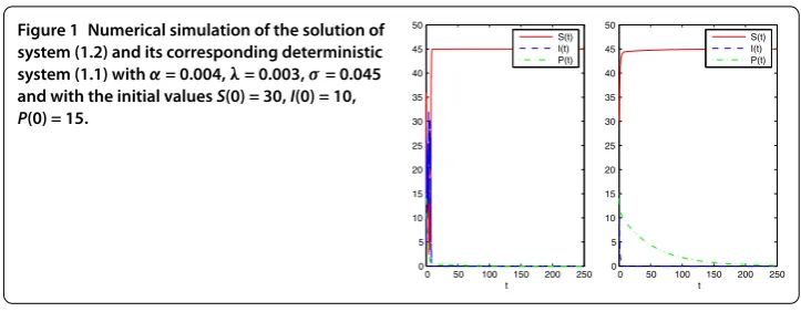
First, we takeα= .,λ= .,σ= .. In this case,
α= . < δ
Kθ = ., σ
= . <(r+Kλ)(μ–Kλ)
λK = ..
We can therefore conclude by Theorem . that the equilibriumE= (, , ) of system
(.) is stochastically asymptotically stable in the large. The numerical simulations in Fig-ure support these results clearly.
Noting that
σ= . >max λ
K = .,
λ
μ= .
= .
and
α= . < δ
Figure 1 Numerical simulation of the solution of system (1.2) and its corresponding deterministic system (1.1) withα= 0.004,λ= 0.003,σ= 0.045 and with the initial valuesS(0) = 30,I(0) = 10,
P(0) = 15.
we see that conditions (a) and (c) of Theorem . are satisfied. Therefore, by Theorem ., for the initial valuesS() = ,I() = , andP() = , the solution of system (.) obeys
lim sup
t→∞
logI(t)
t ≤–. < a.s.,
lim sup
t→∞
logP(t)
t ≤–. < a.s.,
lim
t→∞ t
t
S(s)ds= a.s.
The numerical simulations in Figure support these results clearly, illustrating extinction of the infected prey and the predator.
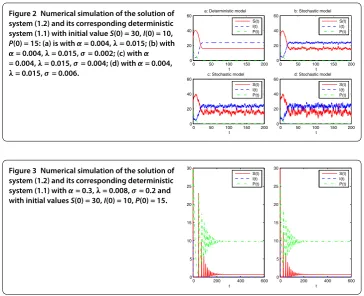
Next, we chooseα= . andλ= .. Then
S=μ
λ = , I=
r( –S K) r K +λ
= .,
and the conditions
μ= . <λK= ., α= . < δ
Kθ = .
are satisfied. Therefore, by Theorem .,P(t) tends to zero exponentially with probability one. We see that the difference between the solution of system (.) andE= (, ., )
in time average is related to the intensity of the white noise. The weaker the white noise, the smaller the difference. The numerical simulations in Figure support these results clearly, illustrating that the solution of system (.) is surroundingE randomly oscillating, and
the extent vibrating enhances gradually with gradual increase ofσ. Finally, we takeα= .,λ= .,σ= .. In this case, we compute
S= δ
θ α = ., P=
r
α
–S K
= .,
δλ
μθ = . <α= ., μ
K = . <λ= .,
σ= . <(βP+μ–λS)
Figure 2 Numerical simulation of the solution of system (1.2) and its corresponding deterministic system (1.1) with initial valueS(0) = 30,I(0) = 10,
P(0) = 15: (a) is withα= 0.004,λ= 0.015; (b) with α= 0.004,λ= 0.015,σ= 0.002; (c) withα = 0.004,λ= 0.015,σ= 0.004; (d) withα= 0.004, λ= 0.015,σ= 0.006.
Figure 3 Numerical simulation of the solution of system (1.2) and its corresponding deterministic system (1.1) withα= 0.3,λ= 0.008,σ= 0.2 and with initial valuesS(0) = 30,I(0) = 10,P(0) = 15.
We can therefore conclude, by Theorem ., that the equilibriumE= (., , .) of
system (.) is stochastically asymptotically stable. The numerical simulations in Figure support these results clearly.
8 Conclusion
In this paper, we have proposed and analyzed an ecoepidemiological model with linear mass-action functional response perturbed by white noise. Based on this model, we mainly have showed that system (.) has a unique positive global solution and investigated how the four equilibriaE,E,E, andEof system (.) will be under stochastic perturbation.
The key parameters are one ecological parameterα, predators’ attack rate on susceptible prey, and one epidemiological parameterλ, the rate of infection.
(i) System (.) is unstable aroundEfor all parametric values. We show that the
equi-libriumEof system (.) is stochastically unstable in Theorem ..
(ii) Ifλ< μK andα<Kδθ, then system (.) is globally asymptotically stable around the equilibriumE. Theorem . shows that ifKλ<μ– λK
σ
(r+Kλ) andα< δ
Kθ, then the
equilib-riumE of system (.) is stochastically asymptotically stable in the large. Theorem .
shows that, under some conditions, the disease will die out, the predator population will go into extinction, and the prey population will approach the carrying capacityK. Bio-logically, it implies that if both the infection rate and the search rate of susceptible prey are low, then the infected prey and predator population cannot survive, and the system converges to the equilibrium where only healthy prey exists.
(iii) Ifλ>Kμ, then the equilibriumEof system (.) exists. Theorem . shows that the
difference between the solution of system (.) andEin time average is only relation with
So there is approximate stability, provided that σ is sufficiently small. Biologically, this implies that if the infection rate is too high and the search rate of susceptible population is moderate, then the predator population cannot survive, and the system converges to the equilibrium where susceptible prey and infected prey coexist in the form of a stable equilibrium.
(iv) Ifλ> μK andα>μθδλ, then system (.) is globally asymptotically stable around the equilibriumE. We also show (Theorem .) that ifλ>Kμ andα>μθδλ, then, under
cer-tain conditions, the equilibriumEof system (.) is stochastically asymptotically stable.
Biologically, it implies that in case of higher infection rate and higher predation rate, all trajectories with the default values converge to the disease-free equilibriumE, where
sus-ceptible prey and predator population coexist in the form of a stable equilibrium.
Appendix 1
In this section, we list some definitions and theory used in the previous sections. In general, consider ad-dimensional stochastic differential equation
dx(t) =fx(t),tdt+gx(t),tdB(t) fort≥t. (A.)
Assume thatf(,t) = andg(,t) = for allt≥t. Sox(t)≡ is a solution of equation
(A.), called the trivial solution or equilibrium position.
Definition A.([]) (i) The trivial solution of system (A.) is said to be stochastically sta-ble or stasta-ble in probability if for every pair ofε∈(, ) andr> , there existsδ=δ(ε,r,t) >
such that
Px(t;t,x)<rfor allt≥t
≥ –ε
whenever|x|<δ. Otherwise, it is said to be stochastically unstable.
(ii) The trivial solution is said to be stochastically asymptotically stable if it is stochasti-cally stable; moreover, for everyε∈(, ), there existsδ=δ(ε,t) > such that
P
lim
t→∞x(t;t,x) =
≥ –ε
whenever|x|<δ.
(iii) The trivial solution is said to be stochastically asymptotically stable in the large if it is stochastically asymptotically stable; moreover, for allx∈Rd,
P
lim
t→∞x(t;t,x) =
= .
Lemma A.(Strong law of large numbers []) Let M={Mt}t≥be a real-valued
contin-uous local martingale vanishing at t= .Then
lim
t→∞M,Mt=∞ a.s. ⇒ tlim→∞ Mt M,Mt
= a.s.
and also
lim sup
t→∞
M,Mt
t <∞ a.s. ⇒ tlim→∞ Mt
Lemma A.([]) If there exists a positive-definite decreasing radially unbounded func-tion V(x,t)∈C,(Rd×[t
,∞];R+)such that LV(x,t)is negative-definite,then the trivial
solution of equation(A.)is stochastically asymptotically stable in the large.
Lemma A.([]) If there exists a positive-definite decreasing function V(x,t)∈C,(Sh× [t,∞];R+)such that LV(x,t)is negative-definite,then the trivial solution of system(A.)
is stochastically asymptotically stable.
Appendix 2: The rest of the proof of Theorem 2.1
LetK=μ+δθ+max{r+Kr,Kr +λ+β,θ(α+β)}Bη+Kσ. Then τk∧T
dVS(t),I(t),P(t)≤
τk∧T
K dt+
τk∧T
σI(t) –S(t)dB(t).
Taking expectations yields
EVS(τk∧T),I(τk∧T),P(τk∧T)
≤VS(),I(),P()+E
τk∧T
K dt
≤VS(),I(),P()+K T. (.)
Setk={τk≤T}fork≥k. Then, by (.),P(k)≥ε. Note that, for everyω∈k, at least one ofS(τk,ω),I(τk,ω), andP(τk,ω) equals eitherkor k, and henceV(S(τk∧T),I(τk∧ T),P(τk∧T)) is no less than either
k– –logk
or
k– –log k =
k– +logk.
Consequently,
VS(τk∧T),I(τk∧T),P(τk∧T)
≥(k– –logk)∧
k– +logk
.
It then follows from (.) and (.) that
VS(),I(),P()+K T
≥Ek(ω)V
S(τk∧T),I(τk∧T),P(τk∧T)
≥ε
(k– –logk)∧
k– +logk
,
Competing interests
The authors declare that they have no competing interests.
Authors’ contributions
The authors have contributed to the manuscript on an equal basis. All authors read and approved the final manuscript.
Author details
1School of Science, Changchun University, Changchun, 130022, China.2Department of Mathematics, Yanbian University, Yanji, 133002, China. 3College of Science, China University of Petroleum (East China), Qingdao, 266580, China.4Nonlinear Analysis and Applied Mathematics (NAAM)-Research Group, King Abdulaziz University, Jeddah, Saudi Arabia.5School of College of Basic Sciences, Changchun University of Technology, Changchun, 130021, China.
Acknowledgements
The work was supported by the Scientific and Technological Research Project of Jilin Province’s Education Department (2015, No. 10; 2014, No. 294), the Education Science Research Project of Jilin Province (No. GH150104), Program for NSFC of China (No. 11371085) and the Fundamental Research Funds for the Central Universities (No. 15CX08011A).
Received: 26 June 2015 Accepted: 28 January 2016 References
1. Hadeler, KP, Freedman, HI: Predator-prey population with parasite infection. J. Math. Biol.27, 609-631 (1989) 2. Beltrami, E, Carroll, TO: Modelling the role of viral disease in recurrent phytoplankton blooms. J. Math. Biol.32,
857-863 (1994)
3. Hethcote, HW, Wang, W, Han, L, Ma, Z: A predator-prey model with infected prey. Theor. Popul. Biol.66, 259-268 (2004)
4. Xiao, Y, Chen, L: Modelling and analysis of a predator-prey model with disease in the prey. Math. Biosci.171, 59-82 (2001)
5. Venturino, E: Epidemics in predator-prey models: disease in the predators. IMA J. Math. Appl. Med. Biol.19, 185-205 (2002)
6. Venturino, E: Epidemics in predator-prey models: disease in the prey. In: Arino, O, Axelrod, D, Kimmel, M, Langlais, M (eds.) Mathematical Population Dynamics: Analysis of Heterogeneity, vol. 1, pp. 381-393. Wuerz Publishing, Winnipeg (1995)
7. Chattopadhyay, J, Arino, O: A predator-prey model with disease in the prey. Nonlinear Anal.36, 747-766 (1999) 8. Chattopadhyay, J, Bairagi, N: Pelicans at risk in Salton Sea - an eco-epidemiological study. Ecol. Model.136, 103-112
(2001)
9. Chattopadhyay, J, Pal, S: Viral infection on phytoplankton zooplankton system - a mathematical model. Ecol. Model.
151, 15-28 (2002)
10. Chattopadhyay, J, Srinivasu, PDN, Bairagi, N: Pelicans at risk in Salton Sea - an eco-epidemiological model-II. Ecol. Model.167, 199-211 (2003)
11. Chattopadhyay, J, Roy, PK, Bairagi, N: Role of infection on the stability of a predator-prey system with several response functions - a comparative study. J. Theor. Biol.248, 10-25 (2007)
12. Ji, CY, Jiang, DQ, Shi, NZ: Multigroup SIR epidemic model with stochastic perturbation. Physica A390, 1747-1762 (2011)
13. Ji, CY, Jiang, DQ, Yang, QS, Shi, NZ: Dynamics of a multigroup SIR epidemic model with stochastic perturbation. Automatica48, 121-131 (2012)
14. Ji, CY, Jiang, DQ: Analysis of a predator-prey model with disease in the prey. Int. J. Biomath.6, 1350012 (2013) 15. Yuan, CJ, Jiang, DQ: Stochastically asymptotically stability of the multi-group SEIR and SIR models with random
perturbation. Commun. Nonlinear Sci. Numer. Simul.17, 2501-2516 (2012)
16. Li, X, Mao, X: Population dynamical behavior of non-autonomous Lotka-Volterra competitive system with random perturbation. Discrete Contin. Dyn. Syst., Ser. A24, 523-545 (2009)
17. Mao, X: Stochastic Differential Equations and Applications. Horwood, Chichester (1997)