Absolute ruin problems in a compound Poisson risk model with constant dividend barrier and liquid reserves

(1)

R E S E A R C H

Open Access

Absolute ruin problems in a compound

Poisson risk model with constant dividend

barrier and liquid reserves

Dan Peng

1*

_{, Donghai Liu}

1

_{and Zhenting Hou}

2

*_{Correspondence:} [email protected] 1_{School of Mathematics and} Computational Science, Hunan University of Science and Technology, Xiangtan, Hunan 411201, P.R. China

Full list of author information is available at the end of the article

Abstract

In this paper, we consider a compound Poisson surplus model with constant dividend barrier and liquid reserves under absolute ruin. When the surplus is negative, the insurer is allowed to borrow money at a debit interest rate to continue the business; when the surplus is below a fixed level, the surplus is kept as liquid reserves, which do not earn interest; when the surplus attains the level, the excess of the surplus over the level receives interest at a constant rate; when the surplus reaches a higher levelb, the excess of the surplus abovebis all paid out as dividends to shareholders of the insurer. We first derive the integro-differential equations satisfied by the

moment-generating function and moment of the discounted dividend payments until absolute ruin. Then, applying these results, we get explicit expressions of them for exponential claims and discuss the impact of the model parameters on the expected dividend payments by numerical examples.

MSC: 91B30

Keywords: absolute ruin; dividend payments; liquid reserve; moment-generating function; interest

1 Introduction

In the classical compound Poisson surplus model,U(t) is given by

U(t) =u+ct–S(t) =u+ct–

N(t)

i=

Xi, t≥,

whereU() =uis the initial surplus,c>  is the premium rate,{N(t),t≥}is a Poisson process with intensityλ> , which denotes the claim numbers in the interval [,t], and

{Xi,i≥} (representing the sizes of claims and independent of {N(t),t≥}) is a

se-quence of independent and identically distributed nonnegative random variables with common distribution functionF(x) =  –F(x), which satisﬁesF() =  and has a mean

μ=_∞F(x)dx> .

In the recent study of risk theory, the classical compound Poisson surplus model has been modiﬁed to adopt economic and ﬁnancial factors such as interest and dividends. The feature of debit interest assumes that the insurer is allowed to borrow money at a

(2)

debit interest rateβ>  to pay claims when the surplus turns negative. As the insurer pays the debts from its premium income, the negative surplus may return to a positive level. When the premium income is not enough to pay the debit interest (that is, the surplus falls below –_βc), the absolute ruin is said to occur. In recent years, the issue of absolute ruin has received considerable attentions in the actuarial literature. See, for example, Embrechts and Schmidli [], Cai [], Yuenet al.[], Wanget al.[], and Yin and Wang []. For exam-ple, Yin and Wang [] study absolute ruin questions for the perturbed compound Poisson risk process with investment and debit interests by the expected discounted penalty func-tion at absolute ruin. On the other hand, even if an insurer invests all his positive surplus into a risk-free asset, in certain condition, only the excess of the surplus over a certain level can receive interest. To adopt a more ﬂexible and tractable model, Embrechts and Schmidli [] investigated the absolute ruin probability for a more complicated risk model. They assumed that the company can borrow money when the surplus is negative and re-ceive interest for capital above a certain level. Furthermore, Caiet al.[] considered the following special model of Embrechts and Schmidli []:

dU(t) =c dt+r(U(t) –)dt–dS(t), U(t)≥ ,

dU(t) =a dt–dS(t),  <U(t) <. (.)

In (.), an insurer’s surplus is below a certain level>  and is kept as liquid reserves. As the surplus attains the level, the excess of the surplus abovewill earn interest at a constant interest forcer> . They studied the Gerber-Shiu function and discussed the impact of interest and liquid reserves on the ruin probability.

On the other hand, the surplus of the insurer with a certain dividend strategy has also been receiving more and more attention, including [, –]. For instance, de Finetti [] studied the dividend strategy in a discrete process. Lin et al.[] investigated the classical risk model with constant dividend barrier and analyzed the Gerber-Shiu dis-counted penalty function at ruin. Albrecher et al. [] considered the distribution of dividend payments in the Sparre Andersen model with constant dividend barrier. Cai

et al. [] considered a more general model that incorporates the notion of thresh-old strategy. Based on the model (.), they assume that if the surplus continues to surpass a higher level b≥ , then the excess of the surplus above b is paid out as dividends to the insurer’s shareholders at a constant dividend rate, and no interest is earned on the surplus over the threshold level b, and they discuss the interactions of the liquid reserve level, the interest rate, and the threshold level in the proposed risk model by studying the expected discounted penalty function and the expected present value of dividends paid up to the time of ruin. More speciﬁcally, they assume that the portion of the surplus is below a present level is liquid, and the amount in excess of this level is invested under a deterministic interest rate. Instead of implementing a threshold in Cai et al.[], Sendova and Zhang [] consider a percentage of the cur-rent surplus of the insurer and also study the expected discounted penalty function at ruin.

(3)

shareholders at a constant dividend ratec+r(b–). The resulting surplus processUb(t)

can be described by

dUb(t) =

⎧ ⎪ ⎪ ⎪ ⎨ ⎪ ⎪ ⎪ ⎩

–dS(t), Ub(t) >b,

(c+r(Ub(t) –))dt–dS(t), ≤Ub(t)≤b,

c dt–dS(t), ≤Ub(t) <,

(c+βUb(t))dt–dS(t), –βc <Ub(t) < ,

(.)

whereUb() =uis the initial surplus,bis the constant level of dividend barrier,β is the

debit interest rate,ris the credit interest,cis the premium rate, andS(t) = _iN_=(t)Xiis the

aggregate Poisson claim-amount process. DeﬁneTb

u=inf{t:Ub(t)≤–_βc}as the time of absolute ruin (Tub=∞ifUb(t) > –_βc for all

t> ). LetD(t) be the cumulative amount of dividends up to timet, andα>  be the force of interest. Then

Du,b=

Tub



e–αtdD(t)

is the present value of all dividends untilT_ub.

In the sequel, we consider the moment-generating function

M(u,y,b) =EeyDu,b_, _–c

β <u≤b,

whereyis such thatM(u,y,b) exists. We denote thenth moment of the discounted divi-dends by

Vn(u,b) =E

Dn_u_,_b, –c

β <u≤b,n∈N.

Note thatV(u,b)≡ and, whenn= ,V(u,b) =V(u,b) is the expectation ofDu,b. We

will always assume thatM(u,y,b) andVn(u,b) are suﬃciently smooth functions inuand

y, respectively.

The rest of the paper is organized as follows. In Section , we get the integro-diﬀerential equations for the moment-generating function and the nth moment of the discounted dividends. In Section , we ﬁnd their explicit expressions for exponential claims and dis-cuss the impact of the model parameters on the expected dividend payments by numerical examples.

2 Integro-differential equations

In this section, we study the moment-generating functionM(u,y,b), which has been dis-cussed in various surplus processes; for example, see Albrecheret al.[], Cheung ()

etc.Similarly, we can analyze the moments ofD(u,b) throughM(u,y,b); sinceM(u,y,b) has diﬀerent paths for –_βc <u≤b, we deﬁne

M(u,y,b) =

⎧ ⎪ ⎨ ⎪ ⎩

M(u,y,b), –_βc <u< ,

M(u,y,b), ≤u<,

(4)

Theorem . M(u,y,b),M(u,y,b),and M(u,y,b)satisfy the following system of

(5)

Lettinghβ(t,u) =ueβt+ce

βt_–

β –u= (c+βu)

eβt_–

β , we observe thathβ(t,u)→ ast→. By Taylor expansion we have

M

ueβt+ce

βt_{– }

β ,ye –αt_,_b

=M(u,y,b) + (βu+c)t∂M(u,y,b) ∂u –αyt

∂M(u,y,b)

∂y +o(t).

Substituting this expression into (.), dividing both sides of (.) byt, and lettingt→, we get (.). Similarly, we obtain (.) and (.).

Whenu= –_βc, absolute ruin is immediate, namely, no dividend is paid, and we obtain (.).

Whenu=b,

M(b,y,b) = ( –λt)ey[c+r(b–)]tMb,ye–αt,b

+λt b–

 M

b–x,ye–αt_,_b_dF₍_x₎

+λt b

b–M

b–x,ye–αt_,_b_dF₍_x₎

+λt b+_βc

b

Mb–x,ye–αt,bdF(x)

+λt ∞

b+_βc

dF(x) +o(t). (.)

By similar methods we obtain the following equation from (.):

αy∂M(u,y,b)

∂y =

yr(b–) +c–λM(b,y,b) +λF

b+ c

β

+λ b–



M(b–x,y,b)dF(x) +λ b

b–M(b–x,y,b)dF(x)

+λ b+_βc

b

M(b–x,y,b)dF(x). (.)

Lettingu↑bin (.) and comparing it with (.), we obtain (.).

Next, we prove condition (.). Here we only proveM(–,y,b) =M(,y,b). For ≤ u<, letτ be the time that the surplus reaches for the ﬁrst time from ≤u<. As before, we know thattis the time that the surplus reachesfor the ﬁrst time from ≤u<with no claims. Then, by the Markov property ofUb(t),

M(u,y,b) =EIτ<T_ubeyDu,b₊_E_I_τ ≥Tub

eyDu,b

=EIτ<T_ubM,ye–ατ_,_b₊_P_τ_≥_Tb u

=M(,y,b)Ee–ατ_I_τ_<_Tb u

+Pτ≥Tub

(6)

On the other hand, we have

M(u,y,b)≥E

Iτ<Tub,τ=t

eyDu,b₊_E_I_τ_<_Tb

u

eyDu,b

=EIτ<T_ub,τ=tM,ye–αt_,_b₊_P_τ≥_Tb

u

=M(,y,b)e–αt_P₍_T_>_t_{) +}_P_τ ≥Tub

≥e–(λ+α)t_M

(,y,b) +P

τ≥Tub

, (.)

whereTis the ﬁrst claim time. Asu↑ ,τandtboth tend to zero, andlimu↑P(τ≥

Tb

u) = ; lettingu↑ in (.) and (.), we getM(–,y,b) =M(,y,b).

Further, lettingu↑ in (.),u↓ in (.), and using (.), and then lettingu↑ in

(.),u↓ in (.), and using (.), we get (.).

Remark . When= , the conclusions are consistent with Wanget al.[]. Write

Vn(u,y,b) =

⎧ ⎪ ⎨ ⎪ ⎩

Vn(u,y,b), –βc <u< ,

Vn(u,y,b), ≤u<, Vn(u,y,b), ≤u≤b.

Theorem . The moment of the discounted dividend payments until absolute ruin sat-isﬁes the following integro-diﬀerential equations:

(βu+c)V_n_(u,b) – (λ+nα)Vn(u,b)

+λ u+_βc



Vn(u–x,b)dF(x) = , – c

β <u< , (.)

cV_n_(u,b) – (λ+nα)Vn(u,b) +λ u



Vn(u–x,b)dF(x)

+λ u+_βc

u

Vn(u–x,b)dF(x) =  (.)

for≤u<,and,for ≤u≤b,

r(u–) +cV_n_(u,b) – (λ+nα)Vn(u,b) +λ u–



Vn(u–x,b)dF(x)

+λ u

u–Vn(u–x,b)dF(x) +λ

u+_βc

u

Vn(u–x,b)dF(x) = , (.)

with the following conditions:

Vn

–c

β,b

= , (.)

V_n_(u,b)|u=b=nV(n–)(b,b), (.)

Vn(–,b) =Vn(,b), Vn(–,b) =Vn(,b), (.)

(7)

Proof The proof is obvious and we omit it here.

Corollary . For n= ,we retain the risk process,and indeed(.), (.),and(.)can be simpliﬁed to

(βu+c)V_(u,b) – (λ+α)V(u,b)

+λ u+_βc



V(u–x,b)dF(x) = , –c

β <u< , (.)

cV_(u,b) – (λ+α)V(u,b) +λ u



V(u–x,b)dF(x)

+λ u+_βc

u

V(u–x,b)dF(x) =  (.)

for≤u<,and for ≤u≤b,

r(u–) +cV_(u,b) – (λ+α)V(u,b) +λ u–



V(u–x,b)dF(x)

+λ u

u–

V(u–x,b)dF(x) +λ u+_βc

u

V(u–x,b)dF(x) = . (.)

Correspondingly,the boundary condition can be simpliﬁed to

V

–c

β,b

= , (.)

V_(u,b)|u=b= , (.)

V(–,b) =V(,b), V(–,b) =V(,b), (.)

V_(–,b) =V_ (,b), V_ (–,b) =V_ (,b). (.)

Remark . When= , (.) and (.) are reduced to (.) and (.) of Yuenet al.

[], and (.)-(.) are reduced to (A)-(A) of Yuenet al.[], respectively.

3 Explicit expressions for exponential claims

In this section, we assume thatF(x) =  –e–μx_,_x_{> ,}_μ_{> , namely, the claim size}

distri-butionF(x) is the exponential distribution with meanμ. We obtain explicit expressions of the moment-generating function and higher moments of the discounted dividends.

SubstitutingF(x) =  –e–μx _{into (.), (.), and (.), we obtain:}

(βu+c)V_n_(u,b) = (λ+nα)Vn(u,b)

– λ

μe –uμ

u

–_βc

Vn(x,b)e

x

μ_dx_, _–c

β <u< , (.)

cV_n_(u,b) = (λ+nα)Vn(u,b)

–λ

μe –_μu 

–_βc

Vn(x,b)e

x μ_dx₊

u



Vn(x,b)e

x μ_dx

(8)

for ≤u<and, for ≤u≤b,

By Slater [], p., the solution of this equation is of the form

gn(z) =anz

whereanandanare arbitrary constants,

M(a,v,x) = (v)

(9)

We know that

β on both sides of (.) and substituting (.) and (.) into it, we obtain

(10)

Whenn= , sincea= , we can get explicit values ofa,a, . . . ,a. By (.)-(.) we obtain the following equations:

⎧

Solving this system, we obtain:

⎧

Whenn≥, by (.)-(.) we obtain the following equations:

⎧

Solving this system of equations, we obtain:

(11)

where

An=

(snhn() –hn())esn+ (hn() –snhn())esn h_n_() –snhn()

,

Bn=

(snhn() –hn())snesn+ (hn() –snhn())snesn h_n_() –snhn()

,

Cn=

h_n_(b)hn() –hn()hn(b)

Bn+

h_n_()h_n_(b) –h_n_(b)h_n_()An,

Cn=

h_n_(b)hn() –hn()hn(b)

Bn+

h_n_(b)h_n_() –h_n_()h_n_(b)An.

From (.) anda,ain (.) we can obtainV(b,b) see the following Examples -. Recursively, we can obtain explicit expressions ofVn(u,b),Vn(u,b), andVn(u,b).

We summarize the exact solution forVn(u,b),Vn(u,b), andVn(u,b) in the following

theorem.

Theorem . Suppose that the claim size distribution is the exponential distribution with F(x) =  –e–xμ_._{Then V}

n(u,b)is given by

Vn(u,b) =anhn(u), – c

β <u< ,

Vn(u,b) =anesnu+anesnu, ≤u<, (.)

Vn(u,b) =anhn(u) +anhn(u), ≤u≤b.

Here,a,a, . . . ,aare obtained in(.)for n= ;otherwise,for n≥,an,an, . . . ,an are obtained by(.).

Remark . In fact, we can obtain the following explicit expressions of M(u,y,b),

M(u,y,b), andM(u,y,b):

M(u,y,b) =  +

∞

n= yn

n!anhn(u), –

c

β <u< ,

M(u,y,b) =  +

∞

n= yn

n!

anesnu+anesnu

, ≤u<,

M(u,y,b) =  +

∞

n= yn

n!

anhn(u) +anhn(u)

, ≤u≤b.

At the end of this section, we use the following numerical examples to discuss the impact of the model parameters on the expected dividend payments.

Example  Table  provides numerical results forV(u,b) for variousuandr. We ﬁnd out thatV(u,b) increases as the credit interest or the initial surplus increases.

Example  Table  provides numerical results forV(u,b) for variousuandβ. We ﬁnd

(12)

Table 1 Inﬂuence ofuandronV13(u,b) withb= 2.8,= 1.5,α= 0.03,μ= 1,λ= 1,c= 1.5, β= 0.09

u\r 0.03 0.04 0.05 0.06 0.07 0.08

1.6 27.8537 28.1717 28.4903 28.8095 29.1294 29.4498 1.7 27.9233 28.2420 28.5614 28.8813 29.2018 29.5230 1.8 27.9961 28.3155 28.6355 28.9562 29.2744 29.5992 1.9 28.0719 28.3920 28.7127 29.0340 29.3559 29.6784 2.0 28.1507 28.4714 28.7928 29.1147 29.4372 29.7603 2.1 28.2323 28.5537 28.8756 29.1981 29.5212 29.8449 2.2 28.3167 28.6386 28.9610 29.2840 29.6077 29.9318 2.3 28.4038 28.7261 29.0490 29.3725 29.6965 30.0212 2.4 28.4933 28.8161 29.1394 29.4632 29.7877 30.1127

Table 2 Inﬂuence ofuandβonV13(u,b) withb= 2.8,= 1.5,α= 0.03,μ= 1,λ= 1,c= 1.5, r= 0.04

u\β 0.09 0.10 0.11 0.12 0.13 0.14

1.6 28.1717 27.1050 26.1146 25.1984 24.3525 23.5719 1.7 28.2420 27.1783 26.1906 25.2769 24.4333 23.6549 1.8 28.3155 27.2544 26.2691 25.3577 24.5162 23.7396 1.9 28.3920 27.3332 26.3501 25.4407 24.6010 23.8262 2.0 28.4714 27.4147 26.4334 25.5258 24.6877 23.9144 2.1 28.5537 27.4987 26.5191 25.6129 24.7763 24.0042 2.2 28.6386 27.5851 26.6069 25.7020 24.8666 24.0956 2.3 28.7261 27.6738 29.6968 25.7930 24.9585 24.1884 2.4 28.8161 27.7648 26.7887 25.8857 25.0521 24.2827

Table 3 Inﬂuence ofuandonV₁₃(u,b) withb= 2.8,α= 0.03,μ= 1,λ= 1,c= 1.5,β= 0.09,

r= 0.04

u\ 0.9 1.1 1.3 1.5 1.7 1.9

1.6 20.8956 22.6238 24.9465 28.1717 32.8679 40.2129 1.7 20.9881 22.7109 25.0265 28.2420 32.9245 40.2483 1.8 21.0815 22.7994 25.1086 28.3155 32.9857 40.2906 1.9 21.1756 22.8892 25.1928 28.3920 33.0512 40.3394 2.0 21.2706 22.9803 25.2789 28.4714 33.1211 40.3944 2.1 21.3662 23.0727 25.3669 28.5537 33.1950 40.4556 2.2 21.4625 23.1662 25.4568 28.6386 33.2779 40.5256 2.3 21.5594 23.2608 25.5484 28.7261 33.3545 40.5952 2.4 21.6570 23.3565 25.6417 28.8161 33.4398 40.6732

Table 4 Inﬂuence ofuandbonV₁₃(u,b) with= 1.5,α= 0.03,μ= 1,λ= 1,c= 1.5,β= 0.09,

r= 0.04

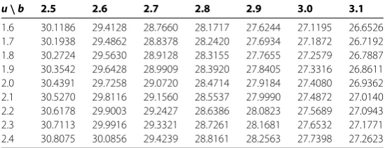
u\b 2.5 2.6 2.7 2.8 2.9 3.0 3.1

(13)

Example  Table  provides numerical results forV(u,b) for variousuand. We ﬁnd out thatV(u,b) increases as the liquid reserve or the initial surplus increases.

Example  Table  provides numerical results forV(u,b) for variousuandb. We ﬁnd out thatV(u,b) decreases asbincreases but increases as the initial surplus increases.

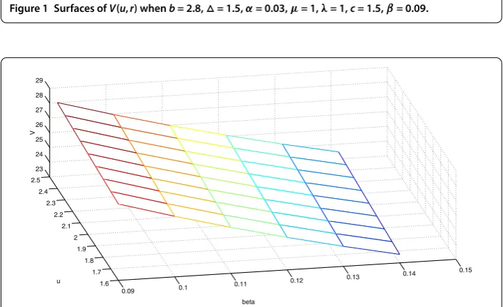
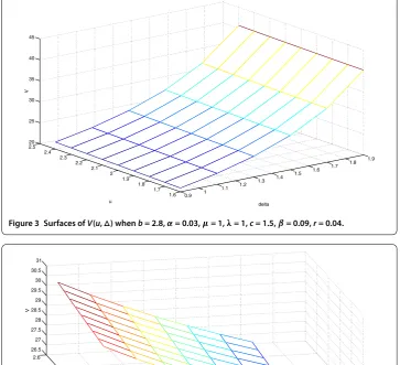
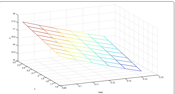
We plot four ﬁgures (Figures -) for the surfaces of the expected dividend payments with the help of Tables -, from which we can see the inﬂuence of credit interest, debit interest, dividend barrierb, and liquid reserveon the values of the expected dividend payments.

For= , our model is reduced to Wang and Yin []. For example, Figures  and  show that the expected dividend paymentsV(u,b) decrease as the debit interest increases but increase as credit interest increases, which is also obtained by Wang and Yin [], Tables  and .

Figure 1 Surfaces ofV(u,r) whenb= 2.8,= 1.5,α= 0.03,μ= 1,λ= 1,c= 1.5,β= 0.09.

(14)

Figure 3 Surfaces ofV(u,) whenb= 2.8,α= 0.03,μ= 1,λ= 1,c= 1.5,β= 0.09,r= 0.04.

Figure 4 Surfaces ofV(u,b) when= 1.5,α= 0.03,μ= 1,λ= 1,c= 1.5,β= 0.09,r= 0.04.

(15)

Figure 6 Surfaces ofV(u,b) when= 0,α= 0.03,μ= 1,λ= 1,c= 1.5,β= 0.09,r= 0.04.

Competing interests

The authors declare that they have no competing interests.

Authors’ contributions

DL conceived of the study and drafted the manuscript, DP participated in the design of the study and made the contribution to simulations. ZH participated in its design and helped to draft the manuscript. All authors have read and approved the ﬁnal manuscript.

Author details

1_{School of Mathematics and Computational Science, Hunan University of Science and Technology, Xiangtan, Hunan} 411201, P.R. China.2_{School of Mathematics and Computational Science, Central South University, Changsha, Hunan} 410075, P.R. China.

Acknowledgements

This research is fully supported by a grant from National Natural Science foundation of Hunan (2015JJ6041), by National Natural Science Foundation of China (11501191), by National Natural Science Foundation of China, Tian Yuan Foundation (11426100), by National Social Science Fund (15BTJ028), and by National Social Science Fund (13BGL106).

Received: 2 July 2015 Accepted: 10 January 2016

References

1. Embrechts, P, Schmidli, H: Ruin estimation for a general insurance risk model. Adv. Appl. Probab.26(2), 404-422 (1994) 2. Cai, J: On the time value of absolute ruin with debit interest. Adv. Appl. Probab.39(2), 343-359 (2007)

3. Yuen, KC, Zhou, M, Guo, J: On a risk model with debit interest and dividend payments. Stat. Probab. Lett.78(15), 2426-2432 (2008)

4. Wang, C, Yin, C, Li, E: On the classical risk model with credit and debit interests under absolute ruin. Stat. Probab. Lett.

80(5-6), 427-436 (2010)

5. Yin, C, Wang, C: The perturbed compound Poisson risk process with investment and debit interest. Methodol. Comput. Appl. Probab.12(3), 391-413 (2010)

6. Cai, J, Feng, R, Willmot, GE: The compound Poisson surplus model with interest and liquid reserves: analysis of the Gerber-Shiu discounted penalty function. Methodol. Comput. Appl. Probab.11(3), 401-423 (2009)

7. Gao, S, Liu, Z: The perturbed compound Poisson risk model with constant interest and a threshold dividend strategy. J. Comput. Appl. Math.233(9), 2181-2188 (2010)

8. Gerber, HU, Shiu, ESW: On optimal dividend strategies in the compound Poisson model. N. Am. Actuar. J.10(2), 76-93 (2006)

9. Lin, XS, Willmot, GE, Drekic, S: The classical risk model with a constant dividend barrier: analysis of the Gerber-Shiu discounted penalty function. Insur. Math. Econ.33(3), 551-566 (2003)

10. de Finetti, B: Su un’impostazione alternativa dell teoria colletiva del rischio. In: Transactions of the XV International Congress of Actuaries, vol. 2, pp. 433-443 (1957)

11. Albrecher, H, Claramunt, MM, Mármol, M: On the distribution of dividend payments in a Sparre Andersen model with generalized Erlang(n) interclaim times. Insur. Math. Econ.37(2), 324-334 (2005)

12. Cai, J, Feng, R, Willmot, GE: Analysis of the compound Poisson surplus model with liquid reserves, interest and dividends. ASTIN Bull.39(1), 225-247 (2009)

13. Sendova, KP, Zang, Y: Interest-bearing surplus model with liquid reserves. J. Insur. Issues33(2), 178-196 (2010) 14. Slater, LJ: Conﬂuent Hypergeometric Functions. Cambridge University Press, London (1960)