R E S E A R C H
Open Access
A low-complexity cell clustering
algorithm in dense small cell networks
Ryuma Seno
1*, Tomoaki Ohtsuki
1, Wenjie Jiang
2and Yasushi Takatori
2Abstract
Clustering plays an important role in constructing practical network systems. In this paper, we propose a novel clustering algorithm with low complexity for dense small cell networks, which is a promising deployment in next-generation wireless networking. Our algorithm is amatrix-basedalgorithm where metrics for the clustering process are represented as a matrix on which the clustering problem is represented as the maximization of elements. The proposed algorithm simplifies the exhaustive search for all possible clustering formations to the sequential selection of small cells, which significantly reduces the clustering process complexity. We evaluate the complexity and the achievable rate with the proposed algorithm and show that our algorithm achieves almost optimal performance, i.e., almost the same performance achieved by exhaustive search, while substantially reducing the clustering process complexity.
Keywords: Cell clustering algorithm, Small cell networks
1 Introduction
In the past few years, fifth generation (5G) wireless communication has become the center of discussion for researchers in this area [1, 2]. 5G is entirely different from conventional standards in that additional improve-ments cannot meet their requireimprove-ments. In addition to the exponential increase in the data amount, the number of wireless devices connected to wireless networks should be considered. As represented by the term “Internet of Things” (IoT), it is predicted that many kinds of devices will operate on wireless networks, which will produce demand for much more network capacity [3].
A simple way to increase the network capacity is nar-rowing the range of cells and increasing the number of cells. Although this method is effective, cell inter-ference becomes more critical when densifying cells with small coverage [4], where radio resource management (RRM) would be of importance for interference mit-igation. RRM schemes are mainly classified into two categories: frequency partitioning schemes and univer-sal frequency reuse schemes. In the former, frequency resources that are orthogonal with each other are assigned
*Correspondence: [email protected]
1Graduate school of Science and Technology, Keio University, 3-14-1, Hiyoshi, Yokohama, Japan
Full list of author information is available at the end of the article
to each cell [5]. On the other hand, in the latter, many cells in the network share the same bandwidth [6]. These schemes may be combined into a hybrid scheme where the network is partitioned into a number of groups of cells and the cells in the same group share the same bandwidth. In [7], the network is classified into two areas, interference-sensitive area (ISA) and not-interference-interference-sensitive area (NISA), and the entire bandwidth is partitioned into two parts, one where interference is tolerated and one where interference is prohibited, which results in the improved frequency utilization efficiency. In this scheme, how to parti-tion the network greatly affects the performance achieved. Ways for interference mitigation are also classified into inter-cell interference coordination (ICIC) and base sta-tion cooperasta-tion (BSC). In ICIC, neighboring cells use the orthogonal bandwidth and avoid the performance degradation of cell-edge users in each cell [8]. In [9], the dynamical management of bandwidth and cluster size results in improved frequency utilization efficiency. On the other hand, in BSC, the neighboring cells share the same bandwidth and cooperate with each other to make the interference beneficial [10]. Since a number of cells coordinate in BSC, the construction of groups in which cells coordinate greatly affects the performance. In both schemes, grouping cells that use the same bandwidth is essential to better performance.
A particular example of a network deployment where inter-cell interference is notably critical is heterogeneous networks (small cell networks) [11]. Network operation by using only macro cells has a capacity hole problem where the achievable rate is extremely low. Small cell net-works are attractive for addressing this problem because small cells can fill the capacity holes. Although small cells can enhance the network capacity, the dense deploy-ment of cells results in severe inter-cell interference. The inter-cell interference problem in small cell networks has been addressed in many studies [12–15, 17, 19]. In [13], semi-distributed interference management in which cell clustering and resource allocation are jointly conducted was proposed for an orthogonal frequency division mul-tiple access (OFDMA)-based two-tier cellular network. In [14], the authors proposed the joint optimization of small cell clustering and a beamforming vector at each base station in dense heterogeneous networks. In [15], inter-ference alignment [16] was utilized as the interinter-ference management technique in heterogeneous networks where inter-tier and intra-tier interferences are eliminated by adequate beamforming and filtering. In [17], the authors proposed a scheme where some available degrees of free-dom (DoF) of macro cells (primary users) were left and utilized for small cells (secondary users) in which interfer-ence alignment was achieved. This enabled the achievable DoF of small cells to be maximized while satisfying the required DoF of macro cells. In [18], clustering was per-formed on the basis of the rate loss caused by cells inter-fering with each other, where the sum of rate loss between cells belonging to different clusters is minimized, which means the rate loss caused by inter-cluster interference is minimized. In [19], the authors proposed clustering small cells in heterogeneous networks where interfer-ence alignment is utilized and found that clustering small cells is effective for improving spectral efficiency normal-ized with the number of antennas at a small cell base station.
The above discussion indicates that “clustering” plays an important role when operating a practical network sys-tem, and a clustering algorithm with lower complexity is desirable. Many kinds of clustering algorithms have been derived in the literature. A most simple clustering algo-rithm is an exhaustive search of all possible clustering patterns (exhaustive algorithm) [20]. Although an exhaus-tive algorithm can achieve global optimal performance, its complexity is significantly high, which is impractical. To achieve a practical clustering algorithm, many stud-ies [21–23] have proposed schemes where each cluster is determined sequentially, i.e., a cluster is determined from cells that have not been selected yet. Papadogian-nis et al. [21], Ng and Huang [22], and Qin and Tian [23] assume wireless networks adopting the coordination between BSs and consider the selection of coordinating
BSs. Papadogiannis et al. [21] proposes changing coordi-nation sets dynamically to fully exploit the macro diver-sity, where each set is determined from BSs which are not selected yet so as to maximize the achievable rate in the set. Ng and Huang [22] consider wireless networks where each user receives the signal from several BSs and pro-pose the cooperative precoding weight design. The set of coordinating BSs is determined so that the BSs within the set interfere with each other most strongly, i.e., each UE selects, at first, the geographically nearest BS and picks up some BSs to which the BS interferes most strongly, where the selected BSs are unified into a coordinating group. Qin and Tian [23] consider, as in [22], to group BSs interfering each other most strongly into a coordination set. In partic-ular, the connectivity between BSs is modeled as a graph whose node corresponds to a BS and the weight of whose edge represents the level of the interference between two BSs and based on the graph the grouping is conducted. A partial graph holding the largest sum of weights among all possible sets, which becomes a coordination set, is separated from the whole graph, and this procedure is sequentially conducted until the grouping is completed. Note that all of these schemes have the feature that each BS cluster is determined sequentially one after another from BSs which are not selected yet. Such schemes are called “greedy algorithms” in general. Although such algo-rithms significantly reduce clustering process complexity, they necessitate sacrificing solution optimality.
In this paper, we propose a novel algorithm for cell clustering. Our algorithm is a matrix-based algorithm where metrics for the clustering process are represented as a matrix on which the clustering problem can be represented as the maximization of elements. In the pro-posed algorithm, we simplify the exhaustive algorithm into sequential selection of small cells through two-step transformations. The clustering problem is divided into some sub-problems each of whose objective function is represented as a sum of elements in the matrix, where each sub-problem corresponds to selecting a small cell. The transformations are conducted to narrow the search range in the same way as the transformation from an exhaustive algorithm to a greedy algorithm where solu-tion optimality is replaced with complexity reducsolu-tion. We evaluate the complexity and the achievable rate per small cell with the proposed algorithm and show that our algorithm achieves almost optimal performance, i.e., almost the same performance achieved in an exhaustive search, while significantly reducing the clustering process complexity.
Finally, Section 5 concludes the paper with a summary of key points.
2 System model
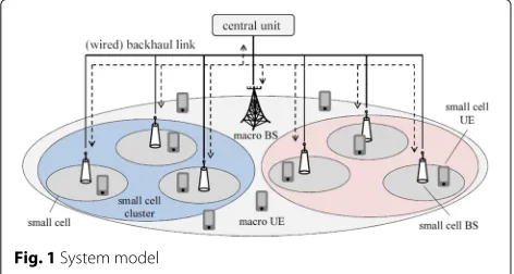
We consider downlink heterogeneous networks where many small cells coexist in a macro cell. The system model is depicted in Fig. 1.
In the macro cell, there areKsmall cells andKmuemacro user equipments (UEs), and in each small cell, there are
Ksuesmall cell UEs. The macro base station (BS) and each small cell BS are respectively equipped with Nmbs and Nsbsantennas, and each UE is equipped withNue anten-nas. Each BS transmitsddata streams to corresponding UE/UEs with spatial multiplexing. Note that in this paper, we assume there is only one macro cell because we focus on the clustering problem of small cells.
Small cells are divided into a number of groups. A clustering formationCis denoted as follows.
C= {C1,C2,. . .,CN} ∈ (1) where Cn denotes thenth cluster, N denotes the num-ber of clusters, and denotes the set of all clustering formations.Cnis further denoted as follows.
Cn= {kn1,k2n,. . .,k|nCn|}, k n
l ∈K (2) where kln denotes the index of the lth small cell in the
nth cluster,|Cn|denotes the number of small cells in the
nth cluster, and K denotes the set of small cells. Note that the clustering formation is determined at a central unit to whom macro BS and each small cell BS connect via wired backhaul link. The required information (the selected clustering pattern, the channel information, etc.) are assumed to be exchanged via the backhaul link without delaying.
A metric is generally defined between cells in the case of cell clustering. There are a number of kinds of metrics, e.g., the distance between cells [22], the effect of mul-tipath fading [24], and signal-to-interference-and-noise ratio (SINR) [25]. In this paper, we denote the metric between small cell i and small cell j by wi,j (∀i,j ∈ K) and ignore the specific definition of the metric. Note that
Fig. 1System model
we assumewi,i = 0 andwi,j = wj,i,∀i,j ∈ K. With the notation of wi,j, the sum of metrics in Cn and the sum of metrics within each cluster under Care respectively represented as follows.
W(Cn) =
i,j∈Cn,i<j
wi,j, (3)
U(C) =
N
n=1
W(Cn)
=
N
n=1
i,j∈Cn,i<j
wi,j. (4)
In general, clustering problems are formalized as the maximization or minimization of the sum of metrics within each cluster. In this paper, without loss of general-ity, we formulate the clustering problem as follows.
C∗=arg max
C∈ U(C) (5)
whereC∗denotes the optimal clustering formation. Although we focus on the clustering problem of small cells in this paper, the proposed algorithm can be eas-ily applied to more general environments, e.g., multi-cell cellular networks or ad hoc sensor networks. In these cases, we only require that appropriate metrics are defined between cells or sensors, likewi,jwhich is defined between small cells in this paper.
The notations in this paper are summarized in Table 1.
3 Proposed method
In the proposed algorithm, metrics between small cells are represented as a matrix on the basis of which we transform the clustering problem. The clustering prob-lem is re-formulated as the maximization of eprob-lements in the matrix, and we transform the exhaustive search of the optimal clustering pattern to the sequential selection of small cells.
3.1 Transformation of clustering process
We divide the metric between small cellswi,jas follows.
wi,j=i,j+j,i (6)
wherei,j denotes the effect of small celljagainst small celli, the SINR or the achievable rate loss, for example. For SINR,i,j indicates SINR at small celliwhen interfered with by small cellj, and for the rate loss,i,jindicates the rate loss at small celliwhen interfered with by small cell
Table 1Notation
Symbol Description
K Number of small cells in a macro cell
N Number of small cell clusters in a macro cell
C A clustering formation∈
Set of clustering formations
Cn nth cluster
kn
l lth small cell innth cluster
K Set of small cells
wi,j Metric between small celliand small cellj i,j Effect from small celljto small celli
W(Cn) Sum of metrics inCn
U(C) Sum of metrics within each cluster underC
Matrix representing metrics
(Ci) Sub-matrix corresponding toCiin
Label based on which elements inare arranged
Xn l
Set of small cells that have been selected
By the(l−1)th cell inCn
Yn Set of small cells that are included in fromC
1toCn
Zn
l Set of small cells inCnup tolth cell
Tn Number of small cells that have been Selected fromC1toCn
We define the following matrix usingi,j.
=
Note that the sum of elements being symmetrical with respect to the diagonal line is the metric between small cells, i.e.,i,j+j,i=wi,j.
On the row and column of the matrix in Eq. (7), small cell indexes are labeled on the basis of which the elements are arranged, i.e., the element in theith row and thejth column in isθi,θj whereθi is theith element in the label. Letdenote the label. In Eq. (7), small cell indexes are labeled as follows.
= {1, 2,. . .,K} (8)
which means that the ith row (and the ith column) is labeled by small celli.
Applying a clustering formationCresults in the change of indexes in, which means the elements are rearranged on the basis of updatedas in Eqs. (10) and (11) where “×” represents the elements that are not included inCn,
∀n. The updated label (C)is represented as follows.
Note that (C)represents the clustering formationC. In the proposed algorithm, we select small cells sequen-tially from the first element ofto the last one, which is equivalent to determining the clustering formation.
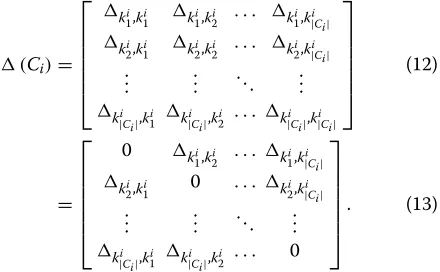
(Ci)represents the matrix corresponding toCiand is denoted as follows.
Based on Eq. (7), the clustering process represented in Eq. (5) is transformed through a two-step transformation as follows.
determination of each cluster in the same way as in a greedy algorithm
• STEP 2 : sequential determination of each cluster is transformed to the sequential selection of small cells
These transformations are conducted to narrow the search range, which results in reduced complexity. In particular, after the step 1 transformation, we determine each cluster sequentially instead of determining all clus-ters together, which means we search for small cells that have not been selected yet when determining a cluster. In addition, after the step 2 transformation, we sequentially determine each small cell instead of each cluster, which further reduces the complexity. By the sequential selection of small cells, we finally derive the clustering formation as represented in Eq. (9).
3.1.1 Step 1
The exhaustive search for all possible clustering forma-tions is formalized as follows using Eqs. (3), (5), and (6).
C∗= arg max Equation (14) is transformed as follows.
arg max
whereYn−1denotes the set of small cells included in from
C1toCn−1.
Equation (16) means that we determine each cluster sequentially, i.e., we search for small cells that have not been selected yet when determining a cluster according to the following equation.
Equation (17) is called greedy algorithm in general.
3.1.2 Step 2
where each symbol represents the group of elements, i.e., the elements that have the same symbol are included in the same group. The division in Eq. (18) is represented mathematically as follows.
From Eqs. (19) and (17) is transformed as follows.
arg max
whereXln−1is the set of small cells that have been selected by the(l−1)th cell inCnand represented as follows.
Therefore, when we determine small cells in Cn, we select small cells sequentially according to the following equation.
Note that Eq. (24) cannot determine the first small cell in each cluster. Hence, we follow the equation below when selecting the first small cell in each cluster.
k1n= arg max k∈K\Yn−1
i∈K\Yn−1
wi,k, n∈ {1, 2,. . .,N}. (25)
Equation (25) means that for the first small cell in each cluster, we select the one that maximizes the sum of met-rics between all small cells that have not been selected yet. Since we do not know which small cells are to be included in the same cluster when selecting the first small cell, it is better to select the one that maximizes the sum of met-rics even if any small cells are selected as the same cluster, which corresponds to Eq. (25).
3.2 Proposed algorithm
Algorithm 1Proposed algorithm
We evaluate the proposed algorithm in terms of two aspects: the complexity of clustering process and the achievable rate per small cell. As mentioned above, there is a trade-off between the complexity and the achievable rate, which means we have to sacrifice the optimality of the solution when reducing the complexity. However, we show that our algorithm is capable of achieving almost optimal performance, i.e., the same performance achieved by an exhaustive algorithm. Therefore, our algorithm can achieve almost optimal performance while reducing the complexity significantly.
In the following, we assume that each cluster comprises the same number of small cells, i.e., the following equation holds.
|Cn| =L, ∀n (26)
whereLdenotes a constant value that holdsLN=K. Note that although there are some specific schemes in the lit-erature [21–23], we exploit the essence of those schemes and refine them into the schemes described in the pre-vious section, i.e., exhaustive algorithm and greedy algo-rithm, when comparing the performance of the proposed scheme, which is more concise.
4.1 Complexity of clustering process
All algorithms in this paper, i.e., exhaustive algorithm, greedy algorithm, and proposed algorithm have the objec-tive function comprising only additions of metrics. There-fore, we use the total number of additions in the clustering process as the complexity. Note that the complexity to calculate the metrics themselves is independent of the clustering algorithm used, which allows us to ignore the complexity for the calculation of the metrics themselves. In the following, we derive the complexity of each algo-rithm quantitatively.
4.1.1 Exhaustive algorithm
Exhaustive algorithm is formalized in Eq. (14) where the objective function is given as Eq. (3). Hence, the number of additions in the objective functionS1eh is expressed as follows.
where the second term in Eq. (27) denotes the number of combinations of two small cells fromCn.
As represented in Eq. (14), the number of operations of the objective function in exhaustive algorithmS2ehis equal to the number of possible clustering formations, which is given as follows.
Therefore, the complexity of exhaustive algorithmSehis given as follows.
From Eq. (29), the order of the complexity is represented as follows.
where the derivation is given in Appendix 1.
4.1.2 Greedy algorithm
Greedy algorithm is formulated as in Eq. (17) where the objective function is given in Eq. (3). Hence, the number of additions in the objective functionS1gd is expressed as follows.
S1gd= L(L−1)
2 . (31)
From Eq. (17), the number of operations of the objective function in greedy algorithmSgd1 is given as follows.
S2gd=
From Eq. (33), we derive the order of the complexity as follows.
O=OL2NL (34)
where the derivation of Eq. (34) is given in Appendix 2.
4.1.3 Proposal
The proposed algorithm is formalized as follows.
kln=arg max k∈K\Xn
l−1
⎧ ⎪ ⎪ ⎪ ⎨ ⎪ ⎪ ⎪ ⎩
i∈K\Yn−1
wi,k, l=1
i∈Zn l−1
wi,k, l=1
. (35)
From Eq. (35), the number of additions in the objective function when selectingklnis given as follows.
S1pr(n,l)=
lK−T(n−1)−1 , l=1
l−1 ,l=1 . (36)
whereT(n−1) denotes the number of small cells selected fromC1toCn−1, i.e.,Tn−1=L(n−1).
The number of operations of the objective function in the proposed algorithm is given as follows.
S2pr(n,l)=K−T(n−1)−(l−1). (37)
Therefore, the complexity of the proposed algorithm is given as follows.
Spr =
N
n=1 L
l=1
Spr1(n,l)×S2pr(n,l)
= 4
3N 3L2−3
2N 2L−3
4N 2L2
+1
4N 2L3+1
2NL− 1 12NL
2+ 1 4NL
3 (38)
whereK=NL.
From Eq. (38), the order of the complexity is derived as follows.
OSpr
=ON3L2+N2L3 (39)
4.1.4 Comparison
We summarize the complexity of each algorithm in Table 2 and show the complexity of each algorithm when
Table 2Complexity of algorithms
Algorithm representationQuantitative representationOrder
Exhaustive
Eq. (29) OL2N(L(N−1)+1) algorithm
Greedy
Eq. (33) OL2NL
algorithm
Proposal Eq. (38) ON3L2+N2L3
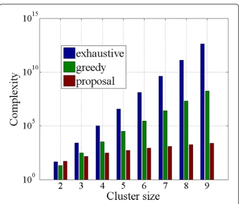
N=3 in Fig. 2 and the complexity of each algorithm when
L=3 in Fig. 3.
As shown in Table 2, the complexity of exhaustive algo-rithm increases exponentially with respect to bothNand
L, which can be verified in Figs. 2 and 3. In terms of greedy algorithm, as shown in Table 2, we found that the complexity increases exponentially with respect toLwhile polynomially with respect toN, which can be verified in Figs. 2 and 3.
Compared to the aforementioned two algorithms, i.e., exhaustive algorithm and greedy algorithm, the complex-ity of the proposed algorithm increases polynomially with respect to bothN andLas shown in Table 2. Therefore, our algorithm reduces the complexity significantly com-pared to the conventional algorithms, particularly whenN
orLincreases.
4.2 Achievable rate
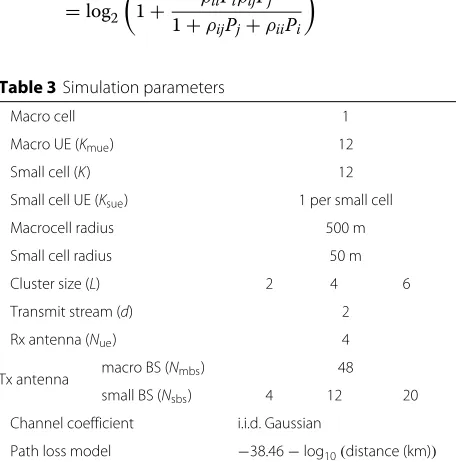
In the work described in this paper, we conducted simu-lations following [19], i.e., precoding (postcoding) weight designs at BS (UE) and the simulation parameters were the same as [19]. The simulation parameters and weight designs are respectively shown in Table 3 and Table 4.
Fig. 3Complexity whenLis fixed to 3
Small cells are uniformly deployed within the circle at whose center the macro BS is located, and each UE is uni-formly deployed within the circle at whose center each corresponding BS is located. The simulation is conducted for each SNR on randomly generated 1000 channel condi-tions. As in [19], the metric between small cells, i.e.,wi,j, is defined as follows.
wi,j=i,j+j,i (40)
wherei,j is the rate loss at small celliwhen interfered with by small celljand given as follows.
i,j=log2(1+ρiiPi)−log2
1+ ρiiPi 1+ρijPj
=log2
1+ ρiiPiρijPj 1+ρijPj+ρiiPi
(41)
Table 3Simulation parameters
Macro cell 1
Macro UE (Kmue) 12
Small cell (K) 12
Small cell UE (Ksue) 1 per small cell
Macrocell radius 500 m
Small cell radius 50 m
Cluster size (L) 2 4 6
Transmit stream (d) 2
Rx antenna (Nue) 4
Tx antenna macro BS (Nmbs) 48
small BS (Nsbs) 4 12 20
Channel coefficient i.i.d. Gaussian
Path loss model −38.46−log10(distance (km))
Table 4Design of weights
Type of weight How to design
Precoding weight Macro BS Direct the null space to macro UEs except for the desired UE and eliminate inter-stream interference
Small BS Align the intra-cluster interference to the strongest interference from macro BS
Postcoding weight Macro UE Eliminate inter-stream interference
Small UE ZF weight nulls out the aligned interference and MMSE weight mitigate the residual interference
where√ρijandPirespectively denote the path loss effect between small BSjand small UEiand the transmit power at small BSi. Note that, as in [19], we assume each small cell BS has the same transmit power, i.e.,Pihas the same value for alli, and we omit the effect of multipath fading in Eq. (41) for the simplicity.
Figure 4 shows the achievable rate per small cell for each cluster size. The x-axis and the y-axis respectively rep-resent SNR and the achievable rate per small cell. Here, “exhaustive” represents the result achieved by exhaustive algorithm, “proposal” represents the result achieved by proposed algorithm, and “random” represents the result obtained when the clustering formation is determine ran-domly. As shown in the figure, “proposal” achieves almost the same rate as “exhaustive,” i.e., almost optimal rate. As mentioned before, since the proposed algorithm reduces the complexity compared to exhaustive algorithm, our algorithm is capable of achieving almost optimal per-formance while reducing the complexity significantly. In addition, it can be found that as the cluster size decreases, the difference between “exhaustive” and “proposal” also decreases. This is because as the cluster size becomes
smaller, the change in the clustering formation becomes less effective with respect to the rate performance.
Figure 5 shows the cumulative distribution function (CDF) of the achievable rate per small cell for each clus-ter size when SNR is 10 and 40 dB. Thex-axis and the
y-axis respectively represent the achievable rate per small cell and CDF. As shown in the figure, as SNR increases the variation of the achievable rate becomes larger. In fact, in the case that the cluster size is 6, although the achiev-able rate takes a value from 1.5 to 2.5 bps/Hz when SNR is 10 dB, it takes a value from 2 to 4 bps/Hz when SNR is 40 dB, where the range of the value becomes twice as large. Therefore, as SNR increases, the change of the clustering formation becomes more effective in the achievable rate.
Although there are some parameters in Table 3, only a few (“macro UE,” “small cell,” and “transmit stream”) can be set arbitrarily and the others should be set to a certain value(s) compulsorily due to the constraint regard-ing, mainly, the calculation of precoding or postcoding weight [19]. In the following, we investigate the perfor-mance when changing these parameters. Note that the cluster size is fixed to 4 unless otherwise specified.
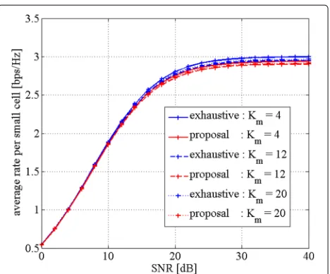
The number of macro UEs: We assume that macro BS
uses the given amount of transmit power to simulta-neously serve macro UEs regardless of the number of macro UEs. Therefore, the total amount of the inter-ference power that the macro BS exerts on small cells remains a certain level regardless of the number of macro UEs, which indicates even if we change the number of macro UEs, the achievable rate per small cell does not change. Fig. 6 shows the achievable rate per small cell ver-sus SNR with different number of macro UEs. Note here that the number of small cells and the number of transmit streams are set to 12 and 2, respectively. As shown in the
Fig. 5CDF of achievable rate
Fig. 6Average rate per small cell with different number of macro UEs
figure, the achievable rate does not change regardless of the number of macro UEs. Note that in the figure Km represents the number of macro UEs.
The number of small cells: With the cluster size fixed,
increasing the number of small cells results in the sev-erer inter-cluster interference because more small cells with fixed cluster size produce more clusters which inter-fere with each other. Therefore, it is easily expected that if we increase the number of small cells the achievable rate decreases and vice versa. Figure 7 shows the achiev-able rate per small cell versus SNR with different number of small cells where the number of small cells is repre-sented as K. Note here that the number of macro UEs
Fig. 8Average rate per small cell with different number of transmit streams
and the number of transmit streams are set to 12 and 2, respectively. As shown in the figure, the achievable rate decreases as the number of small cells increases.
The number of transmit streams: Intuitively, increasing
the number of transmit streams results in the increase of the achievable rate. Figure 8 shows the achievable rate per small cell versus SNR with different number of transmit streams. Note here that the number of macro UEs and the number of small cells are both set to 12. As shown in the figure, the achievable rate increases with the increase of the number of transmit streams.
5 Conclusions
In this paper, we proposed a novel cell clustering algo-rithm that achieves low complexity and high performance. Our algorithm is a matrix-based algorithm where the clustering problem is represented as the maximization of elements in a matrix representing the metric for the clustering process. The algorithm transforms an exhaus-tive search for all possible clustering formations to a sequential selection of small cells, which resulted in sig-nificantly reduced complexity. We evaluated the complex-ity and the achievable rate per small cell and showed that our algorithm achieved almost optimal performance, i.e., almost the same performance achieved by exhaustive search, while significantly reducing the clustering process complexity.
Appendices
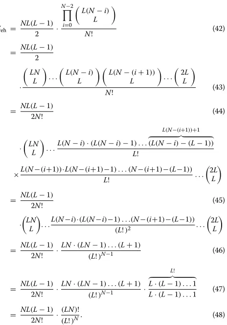
Appendix 1: the derivation of the complexity order for exhaustive algorithm
The complexity represented in Eq. (29) is transformed through Eqs. (42)–(48).
From Eq. (48), we derive the complexity order for exhaustive algorithm as follows.
O(Seh) = O
where we used the following relationship.
O(X!)=OXX. (53)
Appendix 2: the derivation of the complexity order for greedy algorithm
OSgd
where we used the relationship shown in Eq. (53).
Competing interests
The authors declare that they have no competing interests.
Author details
1Graduate school of Science and Technology, Keio University, 3-14-1, Hiyoshi,
Yokohama, Japan.2NTT Network Innovation Laboratories, 1-1, Hikarinooka,
Yokosuka, Japan.
Received: 27 April 2016 Accepted: 31 October 2016
References
1. JG Andrews, S Buzzi, W Choi, SV Hanly, A Lozano, ACK Soong, JC Zhang, What will 5G be? IEEE J. on Sel. Areas in Commun.32(6), 1065–1082 (2014) 2. B Clerckx, A Lozano, S Sesia, 3GPP LTE and LTE-Advanced. EURASIP J. on
Wireless Commun. Netw.2009, 472124 (2009). doi:10.1155/2009/472124 3. A Zanella, N Bui, A Castellani, L Vangelista, M Zorzi, Internet of things for
smart cities. IEEE Internet of Things J.1(1), 22–32 (2014)
4. I Katzala, M Naghshineh, Channel assignment schemes for cellular mobile telecommunication systems: a comprehensive survey. IEEE Pres. Commun.3(3), 10–31 (1996)
5. H-C Lee, D-C Oh, Y-H Lee, inProc. IEEE Int’l Conf. on Commun. Mitigation of inter-femtocell interference with adaptive fractional frequency reuse (IEEE, 2010), pp. 1–5. doi:10.1109/ICC.2010.5502298
6. X Chu, Y Wu, l Benmesbah, B Ling, inProc. IEEE Wireless Commun. Netw. Conf. Workshop. Resource allocation in hybrid macro/femto networks (IEEE, 2010), pp. 1–5. doi:10.1109/WCNCW.2010.5487658
7. H Li, X Xu, D Hu, X Tao, P Zhang, S Ci, H Tang, Clustering strategy based on graph method and power control for frequency resource management in femtocell and macrocell overlaid system. IEEE J. of Commun. and Netw.13(6), 664–677 (2011)
8. G Fodor, inProc. IEEE/ACM Int’l Workshop on Quality of Service. Performance analysis of reuse partitioning technique for OFDM based evolved UTRA (IEEE, 2006), pp. 112–120. doi:10.1109/IWQOS.2006.250457
9. Performance analysis and simulation results of uplink ICIC.Nokia Siemens Networks, 3GPP TSG RAN WG1 #51bis,Spain, Jan 14-18 (2008)
10. H Zhang, B Mehta, AF Molisch, J Zhang, H Dai, inProc. IEEE Int’l Conf. on Commun. On the fundamentally asynchronous nature of interference in cooperative base station systems (IEEE, 2007), pp. 6073–6078. doi:10.1109/ICC.2007.1006
11. V Chandrasekhar, JG Andrews, Femtocell networks: a survey. IEEE Commun. Mag.46(9), 59–67 (2008)
12. N Saquib, E Hossain, L Bao, DI Kim, Interference management in OFDMA femtocell networks: issues and approaches. IEEE Wireless Commun. Mag. 19(3), 86–95 (2012)
13. A Abdelnasser, E Hossain, DI Kim, Clustering and resource allocation for dense femtocells in a two-tier cellular OFDMA network. IEEE Trans. on Wireless Commun.13(3), 1628–1641 (2014)
14. M Hong, R Sun, H Baligh, Z-Q Luo, Joint base station clustering and beamforming design for partial coordinated transmission in
heterogeneous networks. IEEE J. on Sel. Areas in Commun.31(2), 226–240 (2013)
15. W Shin, W Noh, K Jang, H Choi, Hierarchical interference alignment for downlink heterogeneous networks. IEEE Trans. on Wireless Commun. 11(12), 4549–4559 (2012)
16. G Sridharan, Yu Wei, Degrees of freedom of MIMO cellular networks: decomposition and linear beamforming design. IEEE Trans. on Inf. Theory. 61(6), 3339–3364 (2015)
17. D Castanheira, A Silva, A Gameiro, Set optimization for efficient interference alignment in heterogeneous networks. IEEE Trans. on Wireless Commun.13(10), 5648–5660 (2014)
18. S Chen, RS Cheng, Clustering for interference alignment in multiuser interference networks. IEEE Trans. on Veh. Technol.63(6), 2613–2624 (2014)
19. R Seno, T Ohtsuki, J Wenjie, Y Takatori, inProc. IEEE Veh. Technol. Conf. fall. Interference alignment in heterogeneous networks using pico cell clustering (IEEE, 2015), pp. 1–5. doi:10.1109/VTCFall.2015.7390989 20. A Papadogiannis, GC Alexandropoulos, inProc. IEEE Int’l Conf. on Fuzzy Sys.
A value of dynamic clustering of base stations for future wireless networks (IEEE, 2010), pp. 1–6. doi:10.1109/FUZZY.2010.5583933 21. A Papadogiannis, D Gesbert, E Hardouin, inProc. IEEE Int’l Conf. on
Commun. A dynamic clustering approach in wireless networks with multi-cell cooperative processing (IEEE, 2008), pp. 4033–4037. doi:10.1109/ICC.2008.757
22. CTK Ng, H Huang, Linear precoding in cooperative MIMO cellular networks with limited coordination clusters. IEEE J. on Sel. Areas in Commun.28(9), 1446–1454 (2010)
23. C Qin, H Tian, inProc. IEEE Consumer Commun. and Netw. Conf. A greedy dynamic clustering algorithm of joint transmission in dense small cell deployment (IEEE, 2014), pp. 629–634. doi:10.1109/CCNC.2014.6866638 24. K Hosseini, H Dahrouj, R Adve, inProc. IEEE Global Commun. Conf.
Distributed clustering and interference management in two-tier networks (IEEE, 2012), pp. 4267–4272. doi:10.1109/GLOCOM.2012.6503788 25. J-M Moon, D-H Cho, inProc. IEEE Consumer Commun. and Netw. Conf.
Formation of cooperative cluster for coordinated transmission in multi-cell wireless networks (IEEE, 2013), pp. 528–533. doi:10.1109/CCNC.2013.6488494
Submit your manuscript to a
journal and benefi t from:
7 Convenient online submission
7 Rigorous peer review
7 Immediate publication on acceptance
7 Open access: articles freely available online
7 High visibility within the fi eld
7 Retaining the copyright to your article