Volume 2009, Article ID 510617,18pages doi:10.1155/2009/510617
Research Article
Downlink Scheduling for Multiclass Traffic in LTE
Bilal Sadiq,
1Ritesh Madan,
2and Ashwin Sampath
21Wireless Networking and Communications Group, Department of Electrical and Computer Engineering,
The University of Texas at Austin, 1 University Station C0803, Austin, TX 78712-0240, USA
2Qualcomm Flarion Technologies, 500 Somerset Corporate Blvd, Bridgewater, NJ 08807, USA
Correspondence should be addressed to Bilal Sadiq,[email protected]
Received 16 February 2009; Revised 26 June 2009; Accepted 30 July 2009
Recommended by Cornelius van Rensburg
We present a design of a complete and practical scheduler for the 3GPP Long Term Evolution (LTE) downlink by integrating recent results on resource allocation, fast computational algorithms, and scheduling. Our scheduler has low computational complexity. We define the computational architecture and describe the exact computations that need to be done at each time step (1 milliseconds). Our computational framework is very general, and can be used to implement a wide variety of scheduling rules. For LTE, we provide quantitative performance results for our scheduler for full buffer, streaming video (with loose delay constraints), and live video (with tight delay constraints). Simulations are performed by selectively abstracting the PHY layer, accurately modeling the MAC layer, and following established network evaluation methods. The numerical results demonstrate that queue- and channel-aware QoS schedulers can and should be used in an LTE downlink to offer QoS to a diverse mix of traffic, including delay-sensitive flows. Through these results and via theoretical analysis, we illustrate the various design tradeoffs that need to be made in the selection of a specific queue-and-channel-aware scheduling policy. Moreover, the numerical results show that in many scenariosstrict prioritizationacross traffic classes is suboptimal.
Copyright © 2009 Bilal Sadiq et al. This is an open access article distributed under the Creative Commons Attribution License, which permits unrestricted use, distribution, and reproduction in any medium, provided the original work is properly cited.
1. Introduction
The 3GPP standards’ body has completed definition of the first release of the Long Term Evolution (LTE) system. LTE is an Orthogonal Frequency Division Multiple Access (OFDMA) system, which specifies data rates as high as 300 Mbps in 20 MHz of bandwidth. LTE can be operated as a purely scheduled system (on the shared data channel) in that
all traffic including delay-sensitive services (e.g., VoIP or SIP
signaling, see, e.g., [1,2]) needs to be scheduled. Therefore,
scheduler should be considered as a key element of the larger system design.
The fine granularity (180 KHz Resource Block times
1 millisecond Transmission Time Interval) afforded by
LTE allows for packing efficiency and exploitation of
time/frequency channel selectivity through opportunistic scheduling, thus enabling higher user throughputs. However, unlike what is typically the case in wired systems, more capacity does not easily translate to better user-perceived
QoS for delay sensitive flows (VoIP, video-conferencing, stream video, etc.) in an opportunistic system. This is
because a QoS scheduler has to carefully tradeoff
maximiza-tion of total transmission rateversusbalancing of various QoS metrics (e.g., packet delays) across users. In other words, one may need to sometimes schedule users whose delays/queues are becoming large but whose current channel is not the
most favorable; seeSection 2.1for a review and discussion of
results on best effort and QoS scheduling. Therefore, in this
paper, we investigate the case for using queue- and
channel-aware schedulers (see [3–5]) in an LTE downlink to deliver
QoS requirements for a mix of traffic types.
We consider a very general scheduling framework, where
eachflow through its QoS class identifier (see Section 3.2)
is mapped to a set of QoS parameters as required by the scheduler—the mapping can be changed to yield a
different prioritization of flows; this requires no change in
(i) We extend much existing work on single-user queue-and channel-aware schedulers (i.e., schedulers which pick a single user to transmit to in each scheduling interval) to multiuser ones for wideband systems. We also develop a computational architecture which
allows for efficient computation of the scheduling
policies in such a setting. The computational
com-plexity of our scheduler is essentially O(n) for n
users—this complexity is amortized over multiple time steps.
(ii) Through analysis and numerical results for different
traffic models, we illustrate the various design choices
(e.g., the specifics of the tradeoffmentioned earlier
in this section) that need to be made while selecting a scheduling policy. We demonstrate that queue-and channel-aware schedulers lead to significant performance improvements for LTE. Such schedulers not only increase the system capacity in terms of the number of QoS flows that can be supported but also reduce resource utilization. Our simulation method-ology is based on established network evaluation methodologies. We accurately model the LTE MAC layer, and selectively abstract the PHY layer.
While we focus on LTE in this paper, we note that the computational framework and the insights gained via the numerical studies can be extended to other orthogonal division frequency multiple access (OFDMA) technologies such as Worldwide Interoperability for Microwave Access (WiMax) and Ultra Mobile Broadband (UMB).
The rest of the paper is organized as follows. InSection 2, we
provide a representative (but by no means complete) sample of results in literature and relate some of our contributions to the existing work. We also discuss in greater detail the key analytical results on wireless scheduling, and in doing so, make a case for considering queue- and channel-aware
schedulers for both delay sensitive and best effort flows.
The system model—LTE scheduling framework and how various functionalities can and have been used—is presented inSection 3. Having done that, the detailed scheduler design and implementation using fast computational algorithms
is presented in Section 4. Details of simulation setup—
the PHY layer abstraction, network deployment models,
and traffic models—are presented inSection 5. Simulations
demonstrating the performance of the scheduler for various
traffic types, namely, best effort, video-conferencing, and
streaming video, are presented inSection 6. Finally,Section 7
concludes the paper.
2. Scheduling in Wireless Systems:
Prior Work and Discussion
Resource allocation in wireless networks is fundamentally
different than that in wired networks due to the time-varying
nature of the wireless channel [6]. There has been much prior
work on scheduling policies in wireless networks to allocate
resources among different flows based on the channels they
see and the flow state; see, for example, the excellent overview
articles [6,7], and the references therein.
Much prior work in this area can be divided into two categories: scheduling for Elastic (non-real-time) flows, and that for real-time flows.
Scheduling for Elastic (Non-Real-Time) Flows. The end-user experience for an elastic flow is modeled by a concave
increasing utility function of the average rate experienced
by the flow [8]. The proportional fair algorithm (see,
e.g., [9]), where all the resources are allocated to the
flow with the maximum ratio of instantaneous spectral
efficiency (which depends on the channel gain) to the average
rate, has been analyzed in [10–14]. Roughly speaking, this
algorithm maximizes the sum (over flows) of the log of long-run average rates allocated to the flows. For OFDMA-based systems, resource allocation algorithms which focus on maximizing sum rate (without fairness or minimum
rate guarantees) include [15–19]. Efficient computational
algorithms for maximizing the sum of general concave utility functions of the current and/or average rate were obtained
recently in [20].
Scheduling for Real-Time Flows. Real-time flows are typically modeled by independent (of service) random packet arrival processes into their respective queues, and where packets have a delay target, for example, a maximum-delay deadline. Astabilizing scheduling policy in this setting is one which ensures that the queue lengths do not grow without bound.
Stabilizing policies for different wireless network models
have been characterized in, for example, [3–5,21–23]. Under
all stabilizing policies, even though the average rate seen by a flow is equal to its mean arrival rate, still the (distribution
of) packet delay can be very different under different policies
[6]; it is for the same reason that in order to meet the packet
delay/QoS requirement of a real-time flow, it isnotsufficient
to only guarantee the allocation ofat least a minimum average
rate to the flow. Analytical results regarding the queue (or
packet delay) distribution under the schedulers proposed in
[3–5] were recently obtained in [24–26], and are discussed
in the following subsection. For the case where packets are dropped if their delay exceeds the deadline, the scheduling
policy in [27] minimizes the percentage of packets lost.
Work on providing throughput guarantees for real-time
flows includes [28,29], and references therein.
The policies to schedule a mixture of elastic and real-time flows (with delay deadlines of the order of a second)
have been considered in [30] for narrowband systems, and in
[31] for wideband OFDMA systems where the latter assumes
that the statistics of the packet arrival process of the real-time flows along with the channel statistics are known. The
scheduling policy in [31] is persistent and only provides
an average rate guarantee to the real-time flows, which, as
pointed out earlier, is generally not sufficient to guarantee
the packet delay targets. By contrast with the above two, in this paper we investigate whether, given the faster MAC turn-around times and larger bandwidths of LTE systems, the queue- and channel-aware scheduler can and should be used for real-time flows with delay deadlines of few tens of milliseconds. (The answer is yes.)
LTE specifically. The papers that investigate issues similar to
those dealt with in this paper include [32–35]. In [32], it
is shown that adaptive reuse can be beneficial when there is mix of VoIP and data flows, and VoIP is given strictly higher priority. A scheduling policy with strict priority across
classes was also studied by [34]. Within a class, the proposed
scheduling policy computes the resource allocation “chunk-by-chunk” leading to a high computational complexity; the computational complexity of such schedulers can in fact be reduced significantly by using the fast computational
algorithms presented in this paper. The work in [33] showed
that strict prioritization for session initiation protocol (SIP) packets over other packets can lead to better performance. While strict prioritization for low rate flows such as SIP may be feasible, we show that in general it can lead to greatly sub-optimal resource utilization. Specifically, we design scheduling policies where the priority of a class of
flows in notstrictbut ratheropportunistic. The work in [35]
studies a scheduling policy that gives equal priority to all QoS packets until their delay gets close to the deadline; when the packet delays get close to the deadline, the scheduling priority of such packets is increased. In fact, this policy can be seen as belonging to a wider class of queue- and
channel-aware schedulers whichsmoothlypartition the queue or delay
state space in regions where channel conditions are given a higher weight and regions where the delay deadlines are given a higher weight. This is made precise in the following subsection.
Scheduling policies specifically for voice over internet
protocol (VoIP) have been studied in, for example, [36–
38]. Policies for full buffer traffic have been studied in,
for example, [2, 39–44]; many of these papers focus on
modifications to the proportional fair algorithm. A packing algorithm to deal with the constraints on resource assign-ment due to single-carrier FDMA on the uplink was studied
in [45]. Fractional power control and admission control for
the uplink have been studied in [46,47], respectively.
2.1. Discussion. To motivate and put into context the simula-tions presented in this paper, here we summarize some of the key analytical results in the area of opportunistic scheduling.
Through this section, it will suffice to picture a fixed number,
N, of users sharing a wireless channel. Each user’s data
arrives to a queue as a random stream where it awaits transmission/service. The wireless channel is time-varying in that the transmission rates supported for each user vary randomly over time. A scheduling rule in this context selects a single user/queue to receive service in every scheduling instant. However, most of the single-user schedulers can be extended to multiuser versions (for wideband systems) with
some effort; inSection 4.2we present the extensions for the
ones used in this paper.
Among many others mentioned in the previous section,
the work in [48] considers opportunistic scheduling in a
setting where users’ queues are infinitely backlogged (this
full buffer setting is typically used to model elastic or best
effort flows). They identify channel-aware opportunistic
scheduling policies, which maximize the sum throughput (or, more generally, sum of any concave utility function of
user throughput) under various types of fairness constraints.
For example, letxi denote the average rate offered to user
iover a long run (assuming the average exists, which does
under stationary channels and scheduling rules) and any
weightsαi > 0 be given, then a scheduler which maximizes
iαixi is given like this: in any scheduling instant, if the
users’ time-varying channel spectral efficiencies take value
K≡(Ki : 1≤i≤N) (whereKiis the spectral efficiency of
ith user’s channel and is computed from its CQI), schedule a
useri∗satisfying
i∗(K)∈arg max
1≤i≤NαiKi. (1)
Setting 1/αiequal to either the exponentially filtered average
of allocated rate (see xi(t) in (6)) or the long-run average
of spectral efficiency, denoted byKi, yields two versions of
proportional fair (PF) scheduling. With αi = 1/Ki in the
above scheduler, define for later usexPF
i ≡ E[Ki1{i∗(K)=i}],
where expectation is with respect to random K having
the same distribution as the time-varying channel spectral
efficiencies. The missing element in these works is the impact
of queueing dynamics, which certainly cannot be ignored for QoS flows like voice, live and streaming video, and so forth.
Once queueing dynamics are introduced, the oppor-tunistic schedulers that are both queue- and channel-aware can and should be considered. Queue-awareness can be incorporated in a scheduler by, for example, replacing the
fixed vectorα≡(αi : 1≤i ≤N) in (1) with a vector field
α(·) on the state space of queue (or delay). That is, at any
time when users’ queues are in stateq≡(qi: 1≤i≤N) and
their channel spectral efficiencies areK≡(Ki: 1≤i≤N),
schedule a useri∗satisfying
i∗q,K∈arg max
1≤i≤Nαi
qKi. (2)
Queue length qi can be replaced/combined with
head-of-line delay,wi. We enumerate a few reasons why queue- and
channel-aware schedulers should be considered.
(a) Opportunistic schedulers which are solely channel-aware may not even be stable (i.e., keep the users’ queues bounded), unless chosen carefully, for exam-ple, using prior knowledge of mean arrival rates into
the users’ queues. See, for example, [49] which shows
the instability of PF scheduling.
(b) There are queue- and channel-aware schedulers that are throughput-optimal, that is, they ensure the queues’ stability without any knowledge of arrival and channel statistics if indeed stability can be achieved under any other scheduler. Examples are
MaxWeight [3], Exponential (Exp) rule [4], and Log
rule [5], which have the same form as (2). Moreover,
necessary and sufficient conditions on α(·) for the
scheduler in (1) to be throughput optimal have also
been shown [50,51].
(c) Throughput optimal schedulers, along with virtual
token queues, can be used to offer minimum rate
guarantees or maximize utility functions of user
(d) Even if stability of the queues were not a concern, still it is imperative for a QoS scheduler to be both channel- and queue-aware: in order to meet QoS requirements, one may need to sometimes schedule users whose delays/queues are becoming large but whose current channel is not the most favorable.
(e) The work in [53] shows that under aconstantload,
scheduling algorithms that are oblivious to queue state will incur an average delay that grows at least linearly in number of users, whereas, channel- and queue-aware schedulers can achieve an average delay that is independent of the number of users.
Throughput optimal schedulers MaxWeight, Exp rule, and Log rule are defined as follows: when users’ queues are
in stateqand their channel spectral efficiencies areK≡(Ki:
1≤i≤N), schedulers MaxWeight, Exp, and Log rule serve
a useri∗MW,i∗EXP, andi∗LOG, respectively, that is given by
augmented with any fixed tie-breaking rule. Queue length
qican be replaced with head-of-line delay,wi, to obtain the
delay-driven version of each scheduler.
As hinted at by the aforementioned (d), a key chal-lenge in designing a queue- and channel-aware scheduler,
that is, choosing the vector field α(·), is determining an
optimal tradeoff between maximizing current transmission
rate (being opportunistic now) versus balancing unequal
queues/delays(enhancing subsequent user diversity to enable future high rate opportunities, ensuring fairness amongst users, and delivering QoS requirements.) Key optimality properties (beyond and more interesting than stability) can be understood from the way a scheduler makes this
trade-off. Next, we examine how the three throughput optimal
schedulers mentioned earlier make this tradeoff, and relate
it to the known asymptotics of queues/delays under these schedulers.
It can be seen that by settingbi=1/Kifor eachiin (3), all
three schedulers reduce to PF when queue lengths of all users
are equal orfairly close. However, “fairly close” is interpreted
differently by each scheduler. To define this more formally,
assume that users’ channels are stationary random processes and let
tion is with respect torandomKhaving the same distribution
as the time-varying channel spectral efficiencies. Then, in
a stable queueing system under EXP rule, xEXP
i (q) is the
average rate seen by theith user, conditional on queues being
in stateq. For anN=2 user system and parametersa1=a2
in (3),Figure 1illustrates the shape of the set
SPF EXP=
q≥0 :xEXPq=xPF, (5)
that is, the partition of the queue state space where average rate of all users under Exp rule is the same as the average
rate under PF; (setsSPFMW,SPFLOGdefined similarly). With line
{q : q1 = q2}as an axis, the partition SPFMW is a cone, the
partitionSPFEXPis cylinder (with gradually increasing radius),
and partitionSPF
LOGis shaped like a French horn [5].
As the queues move out of the partitions SPF
(·) due to
an increase in q1 and/or decrease inq2, the rate allocation
changes in favor ofq1, that is, each scheduler moves away
from being proportional fair in order to balance unequal
queues (or delays). If q1 continues to increase and/or q2
decrease, each scheduler will eventually schedule only user
1 (wheneverK1=/0): the partition where MaxWeight, Exp
rule, and Log rule schedule only the ith queue (whenever
Ki=/0) is, respectively, illustrated bySMWi ,SEXPi , andSLOGi on
Figure 1.
The exact shape of each partition in terms of width, curvature of boundaries, and so forth, depends on the
parameters in (3) and on the finite set thatK takes values
in (defined by all the available MCSs). However, the shapes
of partitions do not depend on the distribution of randomK
[26]. So these shapes are what an engineer will implicitly or
explicitly design (by choosing a vector fieldα(·) or changing
parameters in (3)) in view of the QoS and rate requirements
of users.
Beyond a visual description of partitions as a cone, cylin-der, French horn, and so forth, the following mathematical
description with useful insights can be given [5]: for any
q>0 and scalars >0 and withbi’s as in (3):
(i)Ni=1bixMWi (sq) is constant ins,
(ii)Ni=1bixEXPi (sq) is decreasing ins, and in the limits →
∞, only the longest queue(s) are scheduled (as long as
their channels are nonzero),
(iii)Ni=1bixLOGi (sq) is increasing ins, and in the limits →
∞, the sum is the maximum possible. For example,
with eachbiset to 1/Kiin (3), lims→ ∞xLOG(sq)=xPF.
This property is called radial sum-rate monotonicity (RSM).
Therefore, as the queues grow linearly, (i.e., scaled up by a constant), Log rule (or any scheduler satisfying RSM)
schedules in a manner that de-emphasizesqueue-balancing
in favor of increasing the total weighted service rate (with
respect to weight vectorb); whereas, the Exp rule schedules
in a manner that emphasizesqueue-balancingat the cost of
total weightedservice rate. Then, it is shown in [25] that Exp
rule minimizes the asymptotic probability of max-queue,
maxiaiqi(t), overflow (or, more precisely, the asymptotic
exponential decay rate of max-queue distribution). Similarly,
Log rule has been shown [26] to minimize the asymptotic
q2
Figure1: Partitions of queue state-space under (a) MaxWeight, (b) Exp, and (c) Log rules.
2.1.1. Use of Queue- and Channel-Aware Schedulers for Elastic
Traffic. Throughput optimal schedulers, like Exp and Log
rules, can also be used for scheduling elastic flows which are
often modeled as full/infinitely backlogged buffers instead of
dynamic queues with random arrivals that are independent of service rate. This is done by using virtual token queues
that are fed by deterministic arrivals at a constant rate λi,
and making scheduling decisions based on the virtual queues
[30, 52]. If token rates λi are feasible (i.e., lie within the
opportunistic capacity region associated with the channel),
then each user i will be offered an average rate xi ≥ λi.
Moreover, if token rates λi are not feasible, then recent
asymptotic analysis of Exp [25] and Log [26] rules show
that the average rates (xi : 1 ≤ i ≤ N) have the following
interesting and desirable properties.
(i) Under Log rule, Ni=1bixi is maximized subject to
xi ≤λi. That is, Log rule splits users in two sets, for
one set of usersxi=λi, whereas for the otherxi< λi,
and the sets are chosen such that the total weighted
rateNi=1bixiis maximized.
(ii) Under Exp rule, variabled >0 is minimized subject
toλi−xi≤d/ai. That is, either each user’s average rate
xi is decremented byd/ai(compared to its required
rate λi), or decremented to 0 (i.e., xi = 0) if the
required rateλiis already less thand/ai.
LTE is a purely scheduled system in that all traffic
with diverse QoS requirements needs to be scheduled. LTE
supports sufficiently short turn-around latency allowing for
some opportunistic scheduling even for delay sensitive traffic
(with delay tolerance of few tens of milliseconds). In this
lies the motivation for simulations presented in Section 6
where we make the case that indeed queue- and channel-aware schedulers can be successfully used for delay sensitive
traffic to increase the number of users that can be supported,
as well as reduce the resource utilization under a given load.
3. System Model
3.1. Terminology. We introduce the following standard 3GPP terminology to be used in the rest of the document:
(i)slot: basic unit of time, 0.5 millisecond,
(ii)subframe: unit of time, 1 millisecond; resources are assigned at subframe granularity,
(iii)eNB: evolved Node B, refers the base station,
(iv)UE, user equipment, refers to the mobile,
(v)PDCCH: physical downlink control channel, physical resources in time and frequency used to transmit control information from eNB to UE,
(vi)PDSCH: physical downlink shared channel, physical resources in time and frequency used to transmit data from eNB to UE,
(vii)CQI: channel quality indicator, measure of the signal
to noise ratio (SINR) at the UE when eNB transmits at a reference power, fed back repeatedly from the UE to the eNB.
3.2. LTE Downlink Scheduling Framework. LTE is an OFDM system where spectral resources are divided in both time
and frequency. A resource block (RB) consists of 180 kHz
of bandwidth for a time duration of 1 millisecond. (Strict
definition of aphysical resource blockin LTE is 180 KHz for
0.5 millisecond (slot), but for the purpose of the simulation this definition is adequate.) Thus, spectral resource
allo-cation to different users on the downlink can be changed
every 1 millisecond (subframe) at a granularity of 180 kHz. If hopping for frequency diversity is enabled, then hopping takes place at 0.5 millisecond point of the subframe (called
slot). We useBto denote the total number of resource blocks
in a single subframe.
LTE features a Hybrid-ARQ mechanism based on incre-mental redundancy. A transport block (consisting of data bytes to be transmitted in a subframe) is encoded using a rate 1/3 Turbo encoder and, depending on the CQI feed-back, assigned RBs, and modulation, the encoded transport block is rate-matched appropriately to match the code rate supported by the indicated CQI. With each subsequent retransmission, additional coded bits can be sent reducing
the effective code rate and/or improving the SINR. Though
ith UE’s PDCCH/PDSCH on
nth H-ARQ process
ith UE’s ACK/NACK for
nth H-ARQ process
ith UE’s earliest possible PDCCH/PDSCH
transmission on
nth H-ARQ process
eNB UE
Figure 2: Downlink scheduling time-line and computational
delays. At time 0 the eNB assigns resources for a first transmission to UEi; the assignment is carried over PDCCH while the actual data is sent over PDSCH, both in subframe 0. ACK/NACK information to convey whether the first transmission was decoded successfully is fed back to the eNB by the UE in subframe 5. Subframe 8 is the earliest possible time when a retransmission (if needed) for this packet can occur.
modulation scheme compared to the first transmission, this flexibility is not exploited in this paper.
Thus, in each subframet, the scheduler grants spectral
resources to users (UEs) for either fresh transmissions, or to continue past transmissions (retransmissions). We assume that each re-transmission of a packet occurs 8 ms (i.e., 8 subframes) after the previous transmission—packets are rescheduled for retransmission until they are successfully decoded at the UE, or the maximum (six) retransmissions have occurred. (LTE allows asynchronous HARQ retrans-missions which means that retransretrans-missions can occur any time after the ACK/NACK is received from the UE. In this paper, we do not exploit this flexibility and operate HARQ synchronously. Retransmissions occur with a delay in multiples of 8 ms.) For a new transmission, a modulation
and coding scheme (MCS) is determined by arate prediction
algorithm which takes into account the most recent CQI report for the UE, and the past history of success/failure of transmissions to this UE—the rate prediction algorithm is
explained inSection 4.1.
The control resources (PDCCH) to convey scheduling grants to the users are time-multiplexed with the resources to transmit data (PDSCH) over the downlink. In particular, each subframe is divided into 14 symbols, of which up to three symbols at the start of the subframe can be used
for control signalling. We do not model thedetails of the
control channel signalling, but we do model the overhead associated with this signalling. Specifically, we assume that
out of S = 14 symbols every subframe,Scont symbols are
used for control signalling. We also model the computational
delays as illustrated inFigure 2.
Downlink scheduling decisions can be made on the basis of the following information for each user.
(i)QoS Class Identifier (QCI). In the LTE architecture downlink data flows from a Packet Gateway (called PDN GW) to eNB and then to the UE (user). The PDN GW to eNB is an IP link and the eNB to UE is over the wireless link. When the logical link from the bearer to the UE is set up (called a bearer), a QoS Class Identifier (QCI) is specified. This defines whether the bearer is guaranteed bit-rate or not, target delay and loss requirements, and so forth. The eNB translates the QCI attributes into logical channel attributes for the air-interface and the scheduler acts in accordance with those attributes. (We use the term user and logical channel interchangeably in this paper as we only state the results with one logical channel per user.)
(ii)CQI.The channel quality indicator (CQI) reports are
generated by the UE and fed back to the eNB in quantized form periodically, but with a certain delay. These reports contain the value of the signal-to-noise and -interference ratio (SINR) measured by the user.
We denote byγi(t) the most recent wideband CQI
value received by the eNB at or before timetfor user
i. The LTE system allows several reporting options
for both wideband (over the system bandwidth) and subband (narrower than the system bandwidth) CQI, with the latter allowing exploitation of frequency selective fading.
(iii)Buffer State. The buffer state refers to the state of
the users’ buffers, representing the data available for
scheduling. We assume that for each useri, the queue
length in (the beginning of) subframe t, denoted
by qi(t) bits, and the delay of each packet in the
queue, withwi(t) ms denoting the delay of
head-of-line packet, is available at the scheduler.
(iv)Phy ACK/NACK. At time t, ACK/NACK for all
transmissions scheduled in subframe (t − 8) are
known to the scheduler.
(v)Resource Allocation History: Scheduling decisions can also be based on scheduling decisions in the past. For example, if a user was allocated multiple RBs over the past few subframes, then its priority at the current subframe may be reduced (even though ACKs/NACKs are still pending). A commonly used
approach is to maintain the average rate, xi(t) at
which a user is served. The average rate is updated
at every timetusing an exponential filter as follows:
xi(t)=(1−τi)xi(t−1) +τiri(t), t=1, 2,. . ., (6)
whereri(t) is the rate allocated to theith user at time
t, andτi ∈(0, 1) is a user specific constant; we refer
4. Scheduler Design for LTE
For each subframet, the scheduler first assigns power and
resource blocks to retransmissions for packets which were
not decoded successfully at time (t−8); the modulation and
coding scheme for a retransmission is kept the same as for the previous transmission. The remaining power and spectral resources are distributed among the remaining users for transmissions of new packets. Specifically, each assignment consists of the following:
(i) the identity of the user for which the assignment is made,
(ii) the number of RBs assigned, (iii) the transmission power for each RB,
(iv) the modulation and coding scheme for packet trans-mission.
In this paper, we present the schedulers and fast compu-tational algorithms for the case where power is distributed uniformly across RBs and only the wideband CQI is being reported. However, the schedulers can be extended to case where one or both of the above restrictions are removed. More specifically, each scheduler is described as a solution to an optimization problem, where the optimization problem can be readily extended to the case where one or both of the above restrictions are removed. Moreover, fast computa-tional algorithms to solve these more complex optimization
problems are presented in [20]. Finally, we note that while we
model the overhead for the control channel PDCCH, we do not study algorithms for control channel format selection.
We break the scheduling algorithm into two parts. (a)Rate Prediction. The rate prediction algorithm maps
(based on past history of transmissions for a UE) the CQI reports to a modulation and coding scheme that targets successful decoding in a specified number of transmissions of a packet. Even though a UE repeatedly sends CQI reports to the eNB, still rate prediction is essential in order to account for the uncertainty in the channel gain to the UE. This uncertainty arises due the following reasons:
(i) wireless channels are time-varying,
(ii) CQI is quantized to 4 bits and the quantized value may be too pessimistic (or optimistic), (iii) CQI reports received by the eNB from a UE may
be based on the channel state a few subframes earlier,
(iv) multiple retransmissions of a packet through H-ARQ may be desired to take advantage of the time diversity, where the channel can vary across the retransmissions.
(b)Resource Assignment. Given an achievable spectral
efficiency as determined by the rate prediction
algo-rithm, the resource allocation for new transmissions is determined as a solution of a constrained optimiza-tion problem. The optimizaoptimiza-tion problem depends on the scheduling policy (proportional fair, Exponential rule, etc.).
4.1. Rate Prediction. Rate prediction is the task of deter-mining and adapting to channel conditions, the mapping of reported CQI to the selected transport format. We start
with a baseline mapping (subsequently denoted by f) that
is optimal under AWGN channel. That is to say, assuming
the channel gain is known andstatic, we optimize transport
format for a fixed number of resources, such that the data packet is transmitted successfully to the UE in any targeted number of transmissions. The baseline mapping that is optimal for a static channel may no longer be so for a fading channel because the channel gain from an eNB to a UE can vary from one H-ARQ transmission to the next. Hence, the selection of the transport format has to take into account this uncertainty or variation in channel gains. One method
of doing this is to use alink marginorbackofffactor, that is
adapted in a closed loop for each link individually, to adjust the transport format from that of the baseline.
Specifically, ifith user’s CQI isγi(t), the user is allocated
bi(t) RBs at time t, and has a termination target (for
successful decoding of the packet at the UE) of Ti
H-ARQ transmissions, then let f(γi(t),bi(t),Ti) denote the
maximum number of bits that can be transmitted over a
static AWGN channel with SINR γi(t). Then for a fading
channel, we select the number of bits as
fγi(t)−δi(t),bi(t),Ti
, (7)
whereδi(t) is the backofffactor. The spectral efficiency (in
bps/RB) for useriis then given by
Ki(t)= f
as described in what follows. If theith user’s transmission is
indeed decoded correctly in (or under) the targeted number
of transmissions, Ti, then δi is decremented (to at most
δMIN= −15 dB) by some fixed smallε(dB), that is,
δi(t+ 1)=max(δi(t)−ε,δMIN). (9)
If, however, the transmission is decoded in more than Ti
number of transmissions (or not decoded at all), thenδiis
incremented (to at mostδMAX=15 dB) bysεfor some fixed
s≥1, that is,
δi(t+ 1)=min(δi(t) +sε,δMAX). (10)
We note that the above rate prediction algorithm is fairly
standard and has been studied in detail in [54].
For best effort flows,Tiis not fixed over time: it is set to
3 unless (i)γi(t) is so high that settingTi to a lower value
results in more than 20% increase in spectral efficiencyKi(t)
(in which caseTi is chosen to maximizeKi(t)), (ii)γi(t) is
too low forTi = 3 to be feasible (in which caseTiis set to
the smallest feasible value). This allows for a high granularity
in picking a spectral efficiency as well as for taking advantage
of time diversity. For delay sensitive flows,Tiis always set to
4.2. Scheduling Policies. In this subsection, we describe the schedulers used for simulation results presented in Section 6, whereas, the fast computational algorithms for these schedulers are presented in the following subsection.
Best effort flows are scheduled using a utility maximizing
scheduler, whereas, QoS flows are scheduled using Exp rule,
Log rule, or Earliest-Deadline-First (EDF). An efficient
com-putational architecture to compute the resource allocation corresponding to a subset of these policies is presented in the following subsection.
4.2.1. Utility Maximizing Scheduler for Best Effort. Recall that
xi(·) denotes the exponentially filtered average rate of useri,
that is,
xi(t+ 1)=τiKi(t)bi(t) + (1−τi)xi(t), (11)
whereKi(t) is defined in (8),τi∈(0, 1) is a parameter,bi(t)
is the number of RBs allocated to useriin subframet, and
xi(0) = 0. We setτi = 1/500 for all users (i.e., the time
constant of the exponential filter for rate averaging is 1/τi=
500 subframe). Moreover, letUi : R+ → R be a concave
continuously differentiable utility function (of average rate
xi) associated with useri. We consider functionsUisuch that,
forxi∈(0,∞), we have
forα = 0. Then in any subframe t, the utility maximizing
scheduler allocates RBsb(t)=(bi(t) : 1≤i≤N), whereN
is the number of users) in order to maximize
N
i=1
Ui(τiKi(t)bi(t) + (1−τi)xi(t)). (13)
We note the following points.
(a) Asα → 0, the scheduler reduces to a proportional
fair scheduler. Specifically, this scheduler will allocate the next fraction of available bandwidth resource to a
user with maximumKi(t)/xi(t).
(b) Asα → 1, this scheduler reduces to max sum-rate
scheduler.
(c) Asα → −∞, it reduces to the max-min fair
sched-uler, that is, it maximizes the minimum average rate.
4.2.2. Delay-Driven Log and Exp Rules. Log and Exp rules used in simulations are similar to the ones introduced in Section 2.1 (see (3)), however, instead of scheduling, one user in every scheduling instant, we can now schedule one user in every RB in the current subframe. So the scheduler makes scheduling decisions one RB at a time, and updates
queues and the buffer state (e.g., head-of-line delay) after
each assignment.
We use the delay-driven version of these rules. Letwi(t)
denote the wait time of the head-of-line packet inith user’s
queue at eNB in subframet. Then under Log rule, in any
subframet,:
(i) the next available RB is allocated to a user i∗(t)
satisfying
i∗(t)∈arg max
1≤i≤Nbilog(c+aiwi(t))×Ki(t), (14)
with ties broken in favor of the user with smallest index,
(ii)qi∗(t) is decremented andwi∗(t) is updated based on
the new buffer state. This is done before the scheduler
computes the optimal user for the next RB.
Parametersbiare set to 1/E[Ki],c=1.1, andai=5/diwhere
di is the 99th percentile delay target of the ith user’s flow.
Recall the setSPF
LOG fromSection 2.1, that is, the partition of state space of delay (or queue) where Log rule and PF take the same scheduling decision. Then the magnitude of vector
a≡(ai: 1≤i≤N) sets thewidthof this partition about the
axis{q≥0 :aiqi=ajqj}.
Exp rule is defined similarly, with (14) appropriately
modified to,
EXP about the axis
{q≥0 :aiqi=ajqj}.
4.2.3. Earliest-Deadline-First Scheduler. This is a queue-aware nonopportunistic scheduler which, in each subframe
t, allocates the next available RB to a user i∗(t) ∈
arg min1≤i≤N(di−wi(t)), and then updateswi∗(t) just as in
the case of Log and Exp rule.
4.3. Efficient Computation of RB Allocation under Various Schedulers. We now describe an efficient computational framework to compute the bandwidth allocations for each
subframe underutility maximization,queue-driven Log, and
queue-driven MaxWeight scheduling policies. We also show how this framework can be used to compute an approximate version of the delay-driven versions.
We first consider a generic optimization problem over the
number of resource blocks,bi(t), allocated to each useri.:
maximize
high enough resource granularity, that is, with appropriate rounding techniques the loss in optimality is negligible. The
maximum bandwidth that can be allocated to useriat timet
is given by
putation of different scheduling policies can be formulated
as the aforementioned optimization problem as follows. (i)Utility Maximization. Here, we definegi(y) as
where we recall thatxi(t) is the average rate allocated
to userias computed by an exponential filter at time
t(see (11)).
(iii)Queue-Driven MaxWeight Rule. In this case, gi is
defined as
The delay-based versions of Log rule and MaxWeight can also be computed by first approximating those as queue-based
rules like this: letλi≡qi(t)/wi(t), that is, the average arrival
rate over the wait time of the head of line packet. Thenwi(t)
in delay-based rules can be substituted withqi(t)/λi.
Define the projection operator overRas
P[a,b]
y=maxminy,b, 0, a,b∈R. (21)
This operator projects a real variable over the interval [a,b].
Necessary and sufficient conditions forb(t) to be optimal
are given by [20]
The followingbisection searchonλcan be used to solve the
aforementioned problem [20]:
Givenλmin=0,λmax=K
1(t)g(K1(t)B), tolerance.
Repeat
(a)Bisect.λ=(λmin+λmax)/2. (b)Bandwidth Allocation. Compute
bi(t)=P[0,bmax
In practice, about 10 iterations are sufficient to obtain a
solution for an accuracy required for scheduling in LTE. An
exact complexity analysis, and the choice of the tolerance
to compute a solution within a certain bound of the optimal
objective function are possible [20].
User
Figure 3: Equivalent schedules, (a) requires 9 grants versus 5
required by (b).
4.4. Further Reduction of Computation by Optimizing over a Horizon. The computational burden of above algorithms
(especially for large N and B) can be reduced further by
solving the convex optimization for a horizon of a few subframes rather than for each subframe. Specifically, we run the convex optimization and compute the optimal RB allocation to each user—called a user’s RB target—over a horizon of a few subframes (say, 8). Then in each subsequent subframe till the next time the optimization is run, we allocate RBs by only doing the following computations (to fully exploit any CQI variation over the horizon).
(i) Update of QoS metric of users, that is, xi(t), qi(t),
and/or wi(t), based on RB assignments in each
subframe (as they are made).
(ii) Update of spectral efficiency Ki(t) (for users for
which a CQI report was received in the previous subframe).
(iii) Update of users’ priority, that is,dUi/dbi atbi = 0,
once the above two updates have been made. (iv) RBs are first allocated to the highest priority user
till its target is met. If some RBs remain available, they are assigned to next highest priority user, and
so on. Any degenerate cases, like data buffers or
control resources running out are handled such that as many as possible number of RBs are assigned in each subframe.
Remark 1. Beside reducing computational burden, solving the optimization for a horizon has an added advantage of reducing the required control signalling. This is because the a user’s RB-target-over-a-horizon can now be allocated all at once in one subframe (or in a fewer number of subframes) rather than allocating only a few RBs per subframe over
the duration of a horizon. For example, Figure 3 shows
Table1: Simulation Parameters.
Parameter Value Comments
Number of eNBs (3 sectored) 19
19 eNBs in a hexagonal pattern, each with 3 cells and wrap-around was used for full-buffer simulations and to generate the geometry (average SINR) distributions for the QoS simulations
Propagation Model (BTS Ant Ht=32 m, MS=1.5 m)
28.6 + 35 log 10(d) dB,din meters
Modified Hata Urban Prop. Model @1.9 GHz (COST 231 ([59])). Modified means that pathloss is reduced by 3 dB in comparison to COST 231. This is a standard assumption (see, e.g., [58]). Minimum separation between
eNB and UE 35 meters —
Log-Normal Shadowing Standard Deviation=8.9 dB
This shadowing is constant for each UE in each simulation run. The same shadowing amount will be used for all the sector antennas of a BS to a given UE. The correlation coefficient between the eNB’s Tx antennas and a given UE and the eNB’s RX antennas and a given UE is 1.
Shadowing correlation across
cells in an eNB 1 —
Shadowing correlation across
eNBs to a UE 0.5 —
Number of transmit antennas 1 —
Number of receive antennas 1 —
Number of resource blocks 64
This number slightly exceeds the 10 MHz bandwidth and was selected since powers of 2 are convenient when hopping is introduced. It does not change the conclusions about the schedulers. The reader can scale the numbers down to infer exact 10 MHz bandwidth performance.
Number of OFDM symbols per
subframe 14
This is for normal cyclic prefix (CP). Of the 14, the first 3 are assigned to control transmissions (PDCCH, PCFICH and PHICH)
eNB transmit power per cell 20 Watts (43 dBm) — Thermal Noise density −174 dBm/Hz — eNB and UE antenna gains 0 dBi —
Site-to-site distance 2.0 km —
HARQ Synchronous, non-adaptive,
incremental redundancy —
(according to the computed targets) are allocated to the highest priority UE(s). Resultantly, the latter schedule has an advantage of requiring only 5 downlink grants on PDCCH versus 9 required by the former.
5. Simulation Framework
5.1. Network and Deployment Model. The deployment and
channel models are mostly taken from the work in [55–58]
and the relevant parameters are repeated here in Table 1.
For the full-buffer simulation results, two-tiers (19 eNBs, 57
cells) with wrap-around was simulated with users in each eNB modeled explicitly. To save on simulation time, for
the results with QoS traffic (e.g., streaming video or video
conferencing) a step process was followed. First, the two-tier (19 eNBs, 57 cell) scenario was simulated under the assumption that all eNBs were transmitting at full power on the downlink (full loading). This was used to generate the distribution of SINRs (geometries) seen by UEs on the downlink, resulting from pathloss and shadowing.
Wrap-around of cells as outlined in [58] was followed to avoid
edge effects. Second, the center-cell alone was simulated
with data traffic and schedulers, with each UE’s SINR being
drawn from the distribution calculated in the first step. Fast fading (time and frequency selective) was then generated for each UE to determine the instantaneous (per subframe) SINR.
For short-term fading, delay spread, and power-delay
is the classic U-shaped power spectrum that results from Jakes/Clarke’s model. The UE speed simulated was 3 km/h.
The effect of channel estimation error was accounted for by
applying a channel specific backofffactor (such asαterm in
the PHY abstraction modeling section), determined through link-level simulations.
5.2. Physical Layer Modeling. System simulations are con-ducted over a large number of cells/sectors and large number of users. As such, characterizing the channel, the physical layer waveform and/or exact decoding process at short timescales becomes prohibitive in terms of computation and simulation time. Yet, a reasonably accurate behavioral model of the physical layer performance is critically important in obtaining the correct system level performance represen-tation and in tuning MAC/RLC algorithms (such as the scheduler). Link level performance is typically characterized by packet-error-rate (PER) versus long-term average SINR curves, where the latter is computed over all channel realizations. Such a curve is not very useful to use in system level simulations as several critical aspects such as user and channel sensitive rate scheduling, hybrid-ARQ and link adaptation are dependent on the short-term average channel. In some instances, the benefits of MIMO and spatial beamforming would also not be captured (e.g., those schemes often involve dynamic feedback of the spatial channel and subsequent adaptation of antenna weights in accordance), as those too are dependent on the short-term channel realization. Furthermore, one aspect of the system simulation is to allow the tuning of algorithms such as rate prediction, power control, and so forth, and therefore, the dynamic nature of physical layer performance is important
to capture in the system simulation. A number of different
approaches have been proposed and evaluated in the past
(see [60] and references therein for a good summary). In
most instances, an effective SINR that captures the channel
and interference occurrences over all resource elements used
in transmission of the encoded packet, is defined. [60,
Equation (1)] generically defines effective SINR as follows:
SINReff=α1I−1
whereP represents the number of resource elements
(time-frequency resources) used over the packet transmission
thus far, j is the index over the resource elements, SINRj
represents the signal-to-interference and noise ratio on jth
resource element, andI(·) is function that is specific to the
model. Note that if hybrid-ARQ is used, then the summation term should include all the H-ARQ transmissions and
associated resources. The factorsα1andαjallow adaptation
of the model to the characteristics of modulation and coding used as well as any adjustments for coded packet length
relative to a baseline curve. In this paper, we use α1 =
αj = 1 for all j. However, after calculating the effective
SINR as described earlier, adjustments for packet size and channel estimation error are applied. These adjustments are computed using extensive link-level simulations for various fading channels and packet sizes. For the most part, the
sensitivity to packet size is very minor and vanishes for packet
sizes larger than around 500 bits. The work in [60] lists a few
examples for the choice ofI(·) as follows:
I(x)=log2(1 +x),
I(x)=exp(−x),
I(x)=Im(x).
(25)
The first expression represents the unconstrained Gaussian channel capacity, the second is an exponential
approxima-tion called (Effective Exponential SINR metric) and the
last expression usesIm the mutual information at an SINR
x, when modulation alphabet size of m is used. The last
method, called Mutual Information Effective SINR Metric
(MIESM), is widely used and is the method we will use
in this paper. Once we compute the effective SINR per the
above expression, then we look up the AWGN PER versus SINR curve corresponding to that modulation, code rate, and packet size to determine the probability of error. A binary random variable with that probability is then drawn and a corresponding error event is generated.
Few additional points are noteworthy, described as follows.
(i) Even though the aforementioned expressions are indexed by a resource element, in LTE, a resource element represents 1 sub-carrier (15 KHz) over 1 OFDM symbol (approximately 70 microseconds). This represents too fine a granularity and would slow down the simulation. Therefore, we use 1 resource block (180 KHz) over 1 subframe (1 millisecond) as the basic unit for generating the SINR in the simulation. Note that these values would lead to negligible, if any, loss in representation accuracy for practical delay spreads and Dopplers.
(ii) Look-up table is used to calculate the mutual infor-mation indexed by SINR and modulation type. The LTE downlink uses 3 modulation types: QPSK, 16-QAM, and 64-QAM.
(iii) We do not currently model modulation order adap-tation on retransmissions.
(iv) As suggested in [60], a single parameterα1=αj=β
for all jis used. In particular, a value of unity is used
as mentioned earlier, with adjustments for channel estimation error and transport block size.
For CQI reporting, the effective SINR is calculated in
a manner similar to the above, using LTE reference signals
and the constrained capacity. The effective SINR is quantized
to a 4-bit CQI value and fed back to the eNB. The table is generated from link curves in accordance with the block-error rate requirements of the LTE specification.
5.3. Traffic Models. The traffic models used for various
simulations inSection 6 are, namely, full-buffer, streaming
video, and live video. In full-buffer model, as the name
5.3.1. Streaming Video Model. Streaming video model is
borrowed from [61], we summarize it here. Exactly 8 video
packets arrive in a frame length of 100 milliseconds. Then the first arrival time from the beginning of a frame, as well as the seven subsequent interarrival times are independently drawn from a Pareto distribution with exponent 1.2 and truncated to [2.5 milliseconds, 12.5 milliseconds]. Moreover, packet sizes are independently drawn from a truncated Pareto distribution with exponent 0.8. The truncation depends on the desired mean rate, for example, [30, 350] bytes for a mean rate of 90 kbps.
5.3.2. Live Video Model. Live video is modeled as an ON-OFF Markov process. When in ON state, a packet of fixed size is generated every 20 ms. The transition probabilities are such that half the time the process is in ON state. Moreover, mean dwelling time in either state is 2 seconds. Then the parameter which controls the mean rate of a live video flow is the packet size, for example, 1 kilobyte for a mean rate of 200 kbps. This
model is similar to the VoIP model in [61] but with higher
rate due to bigger packet sizes.
6. Simulation Results
In this section, we present the results of a simulation-based evaluation of opportunistic schedulers described in Section 4.2, and discuss the key insights into scheduler design. Three sets of results are presented, each considering a
different model for the arrival traffic into the users’ queues
at eNBs. The three traffic models are, namely, saturated
queues at the eNB, multirate streaming video, and a mix of streaming and live video; the three sets of results are discussed in what follows.
6.1. Queues at eNB Are Saturated. We start by presenting the results for the case where users’ queues at the eNBs are saturated (or infinitely backlogged); these results provide a good comparison and calibration against other published studies.
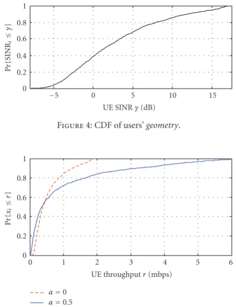
6.1.1. Model. The network deployment model is as described inSection 5.1, with 57 cells (3 per eNB) and 20 users per cell. Figure 4shows the empirical CDF of users’ geometry, that is, users’ SINR induced by the path-loss/shadowing model when all eNBs are transmitting at full power. Each user’s queue at eNB is assumed to be infinitely backlogged, and the transmissions are scheduled according to a utility
max-imizing best effort scheduler described earlier inSection 4.2.
Moreover, to limit the computational burden, the scheduler solves the underlying convex optimization problem once in every 8 subframes over a horizon of 8 milliseconds. Then in each subsequent subframe, the scheduler combines this solution with the current CQI and average rate to compute
a schedule, as described inSection 4.4.
6.1.2. Results and Discussion. The performance measures of interest are the average cell throughput (i.e., cell throughput averaged across all 57 cells) and the distribution of individual
0
Figure4: CDF of users’geometry.
0
UE throughputr(mbps)
α=0
α=0.5
Figure5: Empirical CDFs of average user throughput under best
effort scheduler withα=0 (PF) andα=0.5.
Table2: Fairness versus throughput tradeoffachieved by varyingα.
α Cell thrupt. 5 %-tile throughput 95%-tile throughput 0 1.02 bps/Hz/Cell 134 kbps 1.62 mbps 0.5 1.82 bps/Hz/Cell 48 kbps 4.42 mbps
users’ throughput (i.e., time average of each user’s rate)
under various best effort schedulers, that is, asαassociated
with the utility function varies (seeSection 4.2). Recall that
α → −∞ reduces to max-min fair scheduling, α = 0 to
PF scheduling, andα =1 to max-rate scheduling.Figure 5
shows the empirical CDFs of users’ throughput (rate CDF
for short) for the two cases, α = 0 and α = 0.5, and
Table 2 gives the respective cell throughput as well as the 5 and the 95 percentile read from the two rate CDFs.
Clearly, users’ throughput under the scheduler withα=0 is
morefair than users’ throughput under the scheduler with
α = 0.5, however, this fairness comes at the cost of 44%
drop in the average cell throughput (seeTable 2). Moreover,
from the cross-over point of the two CDFs inFigure 5and
the percentiles inTable 2, as αis increased from 0 to 0.5,
about half the users see a higher throughput (e.g., 3 times higher around the 95 percentile) at the cost of the other half seeing a lower throughput (e.g., 3 times lower around
the 5 percentile). Similarly other tradeoffs between fairness
and cell throughput can be obtained by varying α, or by
6.1.3. Future Work. It is clear that rate CDFs inFigure 5are optimal in that these cannot be dominated by the rate CDFs under any other scheduler (i.e., throughput of a user can only be improved at the cost of that of another). While the above simulation shows that the rate CDF can be controlled to a good degree by varying the utility function, still other more interesting scheduling objectives are, for example,
(i) deliver at least a minimum average ratexito each user
i, or
(ii) maximize a Utility function under minimum and maximum rate constraints.
Both these objectives can be met by devising appropriate utility functions that sharply increase at the minimum rate constraint and saturate at the maximum rate
con-straint. However, as briefly discussed in Subsection 2.1,
these objectives can also be met using queue- and
channel-aware schedulers augmented with virtual token queues.
Such schedulers have been shown to offer greater control
over the rate CDF [30, 52]. It would be interesting to
obtain throughput numbers under these latter scheduling frameworks too.
6.2. Multirate Streaming Video
6.2.1. Model. The deployment model is as described in Section 5.1, with only 1 cell having 20 users. Therefore, the SNRs (induced by the path-loss and shadowing models) of
the 20 users have thesameempirical CDF as the SINR CDF
of users in a multicell system (seeFigure 4). Letγidenote the
SNR (induced by the path-loss and shadowing models) of
useri. We index the users in increasing order ofγi, that is, we
haveγ1< γ2<· · ·< γ20.
Theith user’s queue at eNB is fed by a video stream (see
Section 5.3) with mean rate λi, and the transmissions are scheduled according to EDF, Log, or Exp rules described in Section 4.2. The parameters for each scheduler are fixed for a (soft) 99 percentile packet delay target of 250 milliseconds.
We present results for two different operational scenarios.
(a)Load is 0.50 bps/Hz:λi = 90 kbps fori ∈ {1,. . ., 6}
andλi = 360 kbps fori ∈ {7,. . ., 20}. That is, the
mean rate of the video stream for the six lowest SNR users is 90 kbps, whereas, the mean rate of the video stream for the remaining fourteen users is 360 kbps.
(b)Load is 0.64 bps/Hz:λi = 360 kbps for all usersi ∈ {1,. . ., 20}.
Figure 6 gives the plot of λi for system load given in (a)
andλi for system load given in (b) versusγifor each user
i ∈ {1,. . ., 20}. In order to better picture the system load,
let us define the theoretical throughput xi that each user
i ∈ {1, 2,. . ., 20} will see over an AWGN channel under
equal resource splitting and saturated queues, that is,xi ≡
(Sdata/S)(BW/20)×log(1 +γi); (we note that this is roughly
equal to the throughput users see under PF scheduling
assuming infinitely back logged queues as inSection 6.1, that
is, the gain due to opportunistic PF scheduling evens out
0
Figure6: Mean arrival rates into the queues at eNB for operational
scenarios (a) and (b) versus users’ SNRs induced by path-loss model.
the loss due to the errors and delays in CQI reports as well
as errors in rate prediction).Figure 6also gives a plot ofxi
versusγifori ∈ {1,. . ., 20}. For example, for the 6th user,
rateλ6-case(a) = 90 kbps ≈ 0.09 mbps, rateλ6-case(b) =
360 kbps ≈0.35 mbps and ratex6 = 0.43 mbps are plotted
against SNRγ6=0 dB.
6.2.2. Results and Discussion. Recall that the EDF scheduler is not throughput optimal nor opportunistic. However,
in the case (a) above, each λi is chosen small enough
for EDF scheduler to be stable; this, of course, does not guarantee that EDF will meet the QoS target of having the 99 percentile packet delay of less than 250 milliseconds. (The
vector (λi−case(a) : 1 ≤ i ≤ 20) can be shown to lie
in the capacity region achievable under non-opportunistic schedulers.) In fact, the mean and the 99 percentile packet delays of all users under EDF scheduler turn out to be around 670 milliseconds and 1325 milliseconds, respectively. However, under the opportunistic Log and Exp schedulers,
all users comfortably meet their delay targets:Figure 7shows
the mean and 99 percentile packet delays of each user and overall system under Log and Exp schedulers. The delay target of 250 milliseconds is about ten times the channel coherence time and we see that for a reasonable system load, opportunistic scheduling greatly increases the number of QoS flows that can be admitted; (flows with tighter delay constraints are considered in the following subsection).
The results get more favorable to the Log rule as the system load increases to that mentioned in case (b) above (seeFigure 7). QoS degrades more gracefully under the Log rule, in that 1 user under the LOG rule versus 19 under the Exp rule miss the soft delay target of 250 milliseconds.
However, Exp rule still maintains a lower delay spreadacross
20
Figure 7: Users’ and overall (left) mean delays and (right) 99
percentile delays under LOG and EXP rules for two different system loads. Each (+)-tick represents a user’s delay and legend markers represent overall delays.
minimizes the exponential decay rate of the max-queue
distribution irrespective of the values of parametersai, the
pre-exponent must also be playing a role in determining the systems performance. The actual performance over the region of interest (not the theoretical asymptotic tail)
achieved by the Exp rule is more sensitive to the valuesai.
The RSM property of the Log rule naturally calibrates the scheduler to increased load. So unless parameters can be carefully tuned to possibly changing loads and unpredictable channel capacities, the Log rule appears to be more robust a scheduling policy. Intuitively, this is what one would expect from optimizing for the average/overall versus worst case
asymptotic tail (seeSection 2.1).
Suppose the aforementioned simulations also had best
effort flows which were scheduled only using the resources
spared by the streaming video flows. In that case, it is desirable for a QoS scheduler to meet the delay targets of
streaming flows by utilizing fewer resources.Table 3gives the
resource utilization, that is, average number of RBs allocated to streaming flows per subframe, under each scheduler con-sidered earlier. So, for example, borrowing the cell
through-put figure of 1.02 bps/Hz for PF scheduling fromTable 2, the
total throughput seen by the best effort flows in case (a) can
be expected to be about 2 mbps under the LOG rule which is about 7% higher than that expected under the Exp rule.
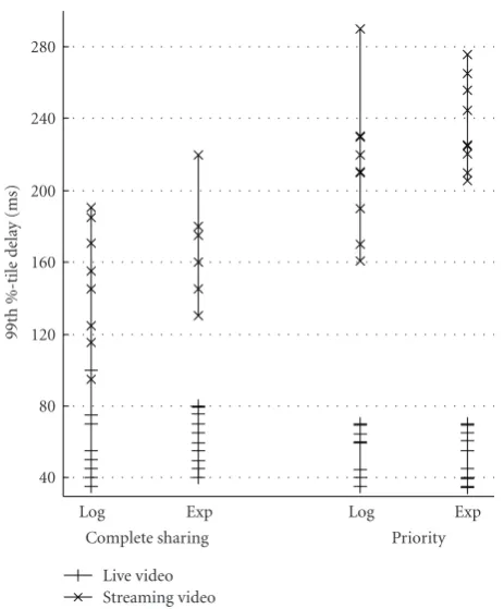
6.3. Mix of Live and Streaming Video
6.3.1. Model. Except for the traffic model, the system is identical to the one described earlier, that is, the streaming
video simulation. The traffic model is as follows. As before,
the users are indexed in increasing order of SNR γi. Then
the queue at the eNB of each (odd) useri ∈ {1, 3,. . ., 19}
is fed by a streaming video source (seeSection 5.3), whereas
the queue for each (even) user j ∈ {2, 4,. . ., 20}is fed by a
live video source. Video rates of each user are described later with the results. The 99 percentile delay target for live video flows is 80 milliseconds, whereas the target for streaming is 250 milliseconds as before. Transmissions are scheduled
according to Log and Exp rules in two different manners.
(i)Strict Priority Given to Live Video Flows. Live video flows are scheduled first (according to Log and Exp rules with parameters set according to the delay target of 80 ms), if any RBs are left over after scheduling the live video flows, those are allocated to the streaming flows (again using Log and Exp rules with parameters set according to the delay target of 250 milliseconds). This scheduling method will be referred to as priority-Exp and priority-Log rules. (ii)All Flows Compete for Resources. Live video flows
are not prioritized in order of scheduling. Setting of scheduler parameters is described later with the results. Since resources are completely shared by the two classes of flows, this scheduling method will be referred to as complete-sharing, and written as cs-Exp and cs-Log rule for short.