R E S E A R C H
Open Access
Existence and persistence of positive
solution for a stochastic turbidostat model
Zuxiong Li
1,2*, Yu Mu
1, Huili Xiang
1and Hailing Wang
1,2*Correspondence:
1Department of Mathematics,
Hubei University for Nationalities, Enshi, Hubei 445000, P.R. China
2School of Mathematics and
Statistics, Huazhong University of Science and Technology, Wuhan, Hubei 430074, P.R. China
Abstract
A novel stochastic turbidostat model is investigated in this paper. The stochasticity in the model comes from the maximal growth rate influenced by white noise. Firstly, the existence and uniqueness of the positive solution for the system are demonstrated. Secondly, we analyze the persistence in mean and stochastic persistence of the system, respectively. Sufficient conditions about the extinction of the microorganism are obtained. Finally, numerical simulation results are given to support the theoretical conclusions.
Keywords: turbidostat model; white noise; persistence in mean; stochastic persistence; extinction
1 Introduction
The continuous culture of microorganism, such as the chemostat and the turbidostat, is a significant way in reality. According to the mechanism of turbidostat, a number of mathe-matical models were introduced to describe the change rate of microorganism and nutri-ent. Herbertet al. [1] constructed the basic model with a constant dilution rate, but they did not give a thorough analysis. Smithet al. [2] completely analyzed the model proposed by [1]. Li [3] introduced a competition turbidostat model with inconstant dilution rate d+k1x1(t) +k2x2(t) and analyzed dynamic behaviors of the system. The above-mentioned systems are often described by ordinary differential equations.
Since the perturbation is inevitable in real conditions, an increasing number of re-searchers have realized that some phenomena, such as time delays [4] and stochastic fac-tors [5], could also cause various dynamical behaviors that are different from the conclu-sions derived from ordinary differential equations. May [5] pointed out that parameters characterizing the natural biological systems have random influence. Mao [6] also em-phasized the significant role of stochastic models in many ways of science and industry. Based on the above tendency and real conditions, the effect of stochastic disturbance on population dynamic has received and has been persistently receiving more attention. In microorganism cultivation, the sense of the stochasticity in the turbidostat may be arisen as a result of the destabilizations such as the uncertainty of the birth rate and the stochastic variations of environmental conditions. In particular, the survival rate is not always equiv-alent to constant due to the feedback phenomenon in the turbidostat. In order to explain those stochastic phenomena, scholars use white noise to represent destabilization from
a biological point of view in generally. Standard Brownian motionB(t) is a reasonable tool to describe the effect of white noise on a dynamic system.
Scholars have studied dynamical behaviors by constructing a stochastic model and ob-tained many important results. Imhofet al. [7] analyzed a deterministic single-substrate model that the dilution rate in the vessel is constant and derived the corresponding con-clusion. They also set up a corresponding stochastic differential equation and investigated the extinction and the persistence of the system. Liuet al. [8, 9] put up a stochastic lo-gistic model and established the sufficient condition of the stability of the positive solu-tion. Campilloet al. [10] built the Fokker-Planck equation of stochastic chemostat and derived an adapted finite difference scheme to approximate the solution of the Fokker-Planck equation. Campilloet al. [11] constructed a set of stochastic chemostat models according to the different population scales and investigated the domain of validity for dif-ferent scales. Zhanget al. [12] proposed a chemostat model with Holling type II functional response and stochastic perturbation and obtained sufficient conditions for the principle of competitive exclusion; they also provided numerical simulation to verify their results by using Milstein’s higher order method. Zhao and Yuan [13] formulated a single-species stochastic chemostat model with periodic coefficients due to seasonal fluctuation; they ob-tained sufficient conditions for the existence of a random positive periodic solution and a globally attractive condition of the random periodic solution. Wanget al. [14] proposed a stochastic chemostat model with periodic wash-out rate and established sufficient condi-tions for the existence of a stochastic nontrivial positive periodic solution for the system. Lvet al. [15] proposed a stochastic competition chemostat model and derived the condi-tions of the threshold between persistence and extinction for the corresponding determin-istic model and the stochastic model, respectively. Menget al. [16] developed a stochastic chemostat model in a polluted environment and obtained the conditions of persistence and extinction for microorganism. They also pointed out that a small enough stochastic disturbance could cause the microorganism to die out even if the microorganism could be persistent in the deterministic model. More mathematical models about microorgan-ism cultivation with constant dilution rate and perturbed phenomena could be found in [17–24]. The study of stochastic population models has been a focus of some scholars in recent years (see [25–41]).
From a biological point of view and real condition, if the concentration of the microor-ganism in the culture vessel is large but the wash-out rate is too small, it will affect the growth of the microorganism in the turbidostat. On the contrary, if the concentration of the microorganism is quite small, the fixed wash-out rate will cause the waste of the nu-trient. Based on the above phenomenon, we construct a turbidostat model with linear wash-out rated+kx(t). Due to the stochastic destabilizations, the maximum growth rate, one of the essential parameters in microorganism cultivation, will undergo variations at different times in the turbidostat. That is, if the birth (death) rate increases (decreases) or the temperature and food are sufficient, the maximum growth rate occurs in advance. If the birth (death) rate decreases (increases) or the temperature and food are insufficient in the system, the maximum growth rate delays. Therefore, the maximum growth rate undergoes a random change.
response. We completely investigate the case that there exists stochastic destabilization for the maximum growth ratem. Therefore, we change the maximum growth ratemin the turbidostat model into a random variablem, in there˜ m˜ =m+αB(t), where˙ B(t) is˙ white noise,i.e., B(t) is a standard Brownian motion defined on a complete probability space (,F,P) (whereFt =σ{(S(t),x(t)); 0≤t≤τe} isσ-filed generated by (S(t),x(t)),
0≤t≤τe).α≥0 represents the intensity of white noise. On the basis of [3, 30] and the
above analysis, we establish the following stochastic turbidostat model: ⎧
⎨ ⎩
dS= [(S0–S)(d+kx) – mS2x
a+S2] dt–αS 2x
a+S2dB(t), dx= [amS+S22 – (d+kx)]xdt+
αS2x a+S2dB(t),
(1.1)
whereSandxrepresent the concentration of the nutrient and microorganism at the time t, respectively.S0 expresses the input concentration of nutrition,d+kxstands for the dilution rate of the turbidostat system. amS+S22 is the Holling III functional response,mis the maximal growth rate andais called the half-saturation constant.S0,d,k,mandaare positive.
This paper is organized as follows. In Section 2, we determine the existence and unique-ness of a positive solution of system (1.1). In Section 3, we further investigate two kinds of persistence of system (1.1) and the extinction of microorganism in the turbidostat and obtain the corresponding break-even concentration. Finally, the effect of white noise on dynamical behaviors of system (1.1) is discussed in detail and specific examples are given to verify our theoretical conclusions.
2 Existence and uniqueness of positive solution
In this section, we demonstrate that system (1.1) has a unique global positive solution. The coefficients of (1.1) are not linear growth, but they are locally Lipschitz continuous. Thus for any initial value (S0,x0)∈R2+, there is a unique positive local solution (S(t),x(t)) ont∈ [0,τe), whereτeis the explosion time [6] (the time that the positive local solution (S(t),x(t))
does not satisfy). If we can show thatτe=∞, then the positive solution (S(t),x(t))∈R2+for allt≥0.
Theorem 2.1 If d>kS0, for any initial value (S0,x0)∈R2+, there is a unique solution (S(t),x(t))of system(1.1)such that(S(t),x(t))∈R2
+for all t≥0almost surely.
Proof On the basis of the definition ofFt, chooseε0> 0 such thatS0>ε0andx0>ε0and
define the stopping timetεas follows:
τε= inf
t∈[0,τe) :S(t,ω)≤εorx(t,ω)≤ε
for anyε≥ε0> 0,
whereτεis a random variable. For anyω∈andε> 0, there existt1,t2, . . . ,tn∈[0,τe)
such thatS(ti,ω)≤ε(i= 1, 2, . . . ,n) orx(ti,ω)≤ε(i= 1, 2, . . . ,n). The stopping timeτε= inf{t1,t2, . . . ,tn}, which meansτεis the first time such thatS(t,ω)≤εorx(t,ω)≤ε.
Throughout this paper, we setinf∅=∞(∅represents the empty set). It is obvious that τεis increasing asε→0. Setτ0=limε→0τε, whenceτ0≤τe a.s. If we can demonstrate
If the above statement is false, then there existδ∈(0, 1) and a constantT> 0 such that P{τ0≤T}>δ. Therefore, we haveP{τε≤T}>δfor all 0 <ε≤ε0.
According to system (1.1), the total biomass in the turbidostat satisfies N(t) =S(t) + x(t)≥0 because of the expression of the Brownian term. Besides,N(t) satisfies the follow-ing equation:
dN(t) =(d+kx)S0–N(t) dt
≤dS0–d–kS0 N(t)dt. (2.1)
Define
dZ(t) dt =dS
0–d–kS0 Z(t)
with the initial valueZ(0) =N(0) =S0+x0. After a simple calculation, it is easy to show that
Z(t) = dS 0
d–kS0+
Z(0) – dS 0
d–kS0
e–(d–kS0)t,
and fort∈[0,τe) we have
Z(t)≤max
S0+x0, dS 0
d–kS0
.
By the comparison theorem for differential equation, we have
N(t)≤Z(t), t∈[0,τe) a.s.
Therefore, we can get that, fort∈[0,τe),
N(t)≤max
S0+x0,
dS0 d–kS0
:=C1.
Define a functionV:R2+→ ¯R+as follows:
VS(t),x(t) = –lnS(t)
C1 –ln x(t)
C1 .
Obviously,Vis nonnegative and definite. Using Itô’s formula, we can obtain
dV=LVdt+αS(x–S) a+S2 dB(t),
where
LV= –S
0(d+kx)
S + 2(d+kx) +
mS(x–S) a+S2 +
1 2
Hence we can use the inequalityN(t)≤C1to conclude that
LV ≤2(d+kx) +mS(x–S) a+S2 +
1 2
α2S2(x2+S2) (a+S2)2
≤2(d+kC1) +mC 2 1
a +
α2C41 a2
:=C2,
which yields the inequality
dV≤C2dt+αS(x–S) a+S2 dB(t).
Integrating both sides for the above inequality from 0 toτε∧T and taking expectation,
we obtain
EVS(τε∧T),x(τε∧T) ≤V(S0,x0) +C2T.
Settingε={τε≤T}for any nonnegativeε≤ε0, we can getP(ε) >δ. In view of the
definition of the stoping time, we conclude, for everyω∈ε, that there exists at least one
ofS(τε,ω),x(τε,ω) is less than or equal toε,
VS(τε),x(τε) 1{ω∈ε}≥–ln
ε
C11{ω∈ε}.
Consequently,
EVS(τε),x(τε) 1{ω∈ε}≥–P(ε)1{ω∈ε}ln
ε C1
> –δln ε
C1,
which yields the inequality
V(S0,x0) +C2T≥EVS(τε),x(τε) 1{ω∈ε}≥–δln
ε C1
.
Whenε→0, we have
V(S0,x0) +C2T→ ∞,
which leads to contradiction with
V(S0,x0) = –lnS0
C1 –lnx0
C1 <∞.
3 Extinction and persistence of the model
Denote
=(S,x)∈R2+:S+x=S0.
For the convenience of demonstration of the main results in this section, we give the following two remarks.
Remark 1 From (2.1), we know that is a nonnegative invariant set for turbidostat stochastic model (1.1), which is essential characteristic for our theoretical analysis in the following section.
Remark 2 Yuanet al. [30] pointed out that ifm≤D(the maximum growth rate is less than or equal to wash-out rate), microorganism in the system must be washed out. Moreover, this conclusion can also be found in [2] (Chapter 1 and Section 4 of Chapter 2) and [7]. If m≤d+kx, the microorganism must be washed out in model (1.1). Thus we always assume m>d+kxin this paper, which meansm>d.
From a biological point of view and the mechanism of turbidostat, if the wash-out rate (the output constant of turbidostat) is larger than the maximum growth rate (the yield constant of turbidostat), there is no microorganism in the culture vessel. In other words, if the maximum growth rate is smaller than the wash-out rate, the population will be extinct. The proof in this section is based onm>d+kx.
On the basis of the positive invariant set ={(S,x)∈R2
+:S+x=S0}, we only need to investigate the following system:
dx=
m(S0–x)2
a+ (S0–x)2– (d+kx)
xdt+ α(S 0–x)2x
a+ (S0–x)2dB(t), (3.1)
with the initial valuex(0) =x0∈(0,S0). We need the following definition and lemma in order to determine the main results.
Definition 3.1([42])
(I) The microorganism in system (1.1) is persistent if
lim
t→∞
1 t
t
0
x(s) ds≥ζ
for some constantζ> 0;
(II) Microorganism in system (3.1) is stochastically persistent in the turbidostat if, for any∈(0, 1), there are positive constantsB1=B1()andB2=B2()such that, for any initial valuex0∈R+,
lim
t→∞infP
x(t)≤B1 > 1 – and lim
t→∞infP
x(t)≥B2 > 1 –.
Lemma 3.1([43]) Let f∈C[[0,∞)×, (0,∞)].If there exist positive constantsλ0andλ such that
logf(t)≥λt–λ0 t
0
for all t≥0,where F∈C[[0,∞)×,R]andlimt→∞F(tt)= 0,a.s.Then
Theorem 3.1 If the break-even concentrationλ1<S0,where
λ1=d(a+ (S 0)2)
mS0 +
α2(S0)3 2m(a+ (S0)2)
for any given initial value(S0,x0)∈R2+,the solution of turbidostat model(1.1)satisfies
lim
which means the microorganism in system(1.1)is persistent.
Proof Define a functionV(x(t)) =lnx(t). Applying Itô’s formula, we have
dV=LVdt+ αS
Integrating (3.2) from 0 tot, we obtain
is the quadratic variation process andYt≤(α(S
0)2
a+(S0)2)4t. Therefore,
lim
t→∞sup
M,Mt
t ≤
α(S0)2 a+ (S0)2
4 <∞.
Using the strong principle of large number, we obtain
lim
t→∞
M(t)
t = 0, almost surely,
and
lim
t→∞
lnx0
t = 0, almost surely.
Ifλ1<S0, we can derive the following result by Lemma 3.1:
lim
t→∞inf
1 t
t
0
x(s) ds≥ maS
0
(a+ (S0)2(2mS0+ka))
S0–λ1 > 0, almost surely.
This completes the proof of Theorem 3.1.
Consider the following time-homogeneous stochastic equation:
dX(t) =bX(t) dt+αX(t) dB(t) withX(0)∈R+.
Lemma 3.2([44]) Let X(t)be a time-homogeneous solution of the above one-dimensional time-homogeneous stochastic equation on E1(one-dimensional Euclidean space).Assume that:
(I) In the domainU⊂E1and some neighborhood thereof,the diffusionα(X)is bounded away from zero;
(II) If,for allX∈E1\U,the mean timeτXat which a path emerging fromXreaches the
setUis finite,andsupX∈KE(τX) <∞for every compact subsetK⊂E1. Then the Markov process X(t)has a stationary distributionπ(x).
Theorem 3.2 If the break-even concentrationλ2<S0,where
λ2=
(a+ (S0)2)d mS0 +
α2(S0)3 m(a+ (S0)2),
for any given initial value(S0,x0)∈R2+,the microorganism x(t)is stochastically persistent in the turbidostat and system(3.1)has a stationary distribution.
Proof Define aC2-functionV:R+→R+for anyp∈(0, 1) as follows:
V(x) = 1
Applying Itô’s formula, one can obtain Multiplying (3.3) byeθtand taking an integration from 0 tot, we obtain
1 tation on both sides of (3.4), we conclude that
LetB1=S0, we have the following equality:
Px(t)≤B1 =Px(t)≤S0 = 1≥1 –,
on the positive invariant set . Moreover, applying Chebyshev’s inequality [6], we obtain
PB2≤x(t) =P
Therefore, the microorganism is stochastically persistent in the turbidostat. Next we prove that system (3.1) has a stationary distribution. Letε> 0 be a small enough number andU be a bounded open subset with a regular boundary such that
which yields that (II) in Lemma 3.2 holds. It is easy to check that the diffusion σ(x) =
α(S0–x)2x
a+(S0–x)2 in system (3.1) is bounded away from zero forx∈(0,S0). Therefore, system (3.1) has a stationary distribution. This completes the proof of Theorem 3.2.
Theorem 3.3 Ifα42 +kS0<d–am+((SS00))22,then for any initial condition(S0,x0)∈R2+,the mi-croorganism x(t)will be extinct with probability one in the turbidostat.
Proof Defining aC2-functionV(x(t)) =lnx(t), we obtain the following equality by Itô’s formula:
By equation (3.5), we define
h(S) = mS 2
a+S2 –d–kx– α2S4 2(a+S2)2.
Forh(S), we can obtain
h(S)≤ α
By equations (3.5) and (3.6), we see that
lnx(t) –lnx0=
which yields the inequality
lnx(t)
0< 0, almost surely. (3.9)
That is, the microorganismx(t) in the vessel will exponentially tend to zero. The proof of
Theorem 3.3 is completed.
4 Discussion and numerical simulation
stochastic phenomena such as the birth rate and the variation of environment. We show that oscillations may occur for system (1.1) when white noise exists. Under the condition of white noise and the feedback control of the turbidostat, system (1.1) may be persistent (stochastically persistent) as described by Theorem 3.1 (Theorem 3.2), and it has a sta-tionary distribution. On the contrary, the microorganismx(t) in the turbidostat might be extinct as displayed by Theorem 3.3 because of white noise and the feedback control of the turbidostat. We explicitly discuss those phenomena with the following three examples, respectively.
Computer simulation of the path of (S(t),x(t)) is provided with the initial value (S(0),x(0)) = (0.4, 0.37). LetS0= 0.77,d= 0.18,k= 0.2,m= 1.6,a= 1.7, and chooseα= 0 orα= 0.3.
⎧ ⎨ ⎩
dS(t) = [(0.77 –S(t))(0.18 + 0.2x(t)) –1.61.7+S2(St2)(xt()t)] dt–0.3S 2(t)x(t) 1.7+S2(t) dB(t), dx(t) = [1.7+1.6SS22(t(t))– (0.18 + 0.2x(t))]x(t) dt+
0.3S2(t)x(t) 1.7+S2(t) dB(t).
(4.1)
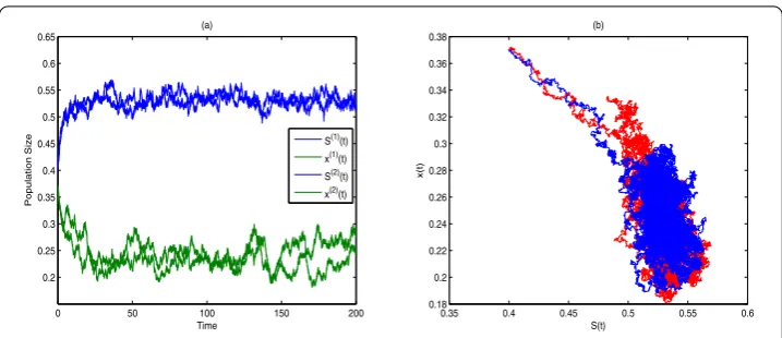
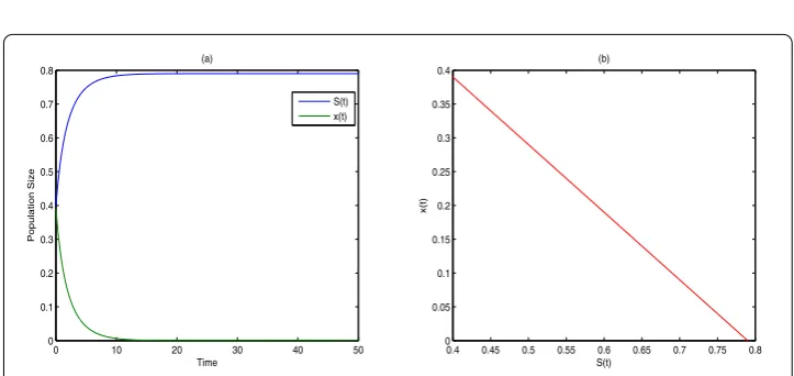
Whenα= 0, system (4.1) becomes a corresponding deterministic model. Figure 1 de-picts the persistence of microorganism in the deterministic model. Whenα= 0.3, which means system (4.1) has stochastic destabilization from internal or external factors, the break-even concentration
λ1=
(a+ (S0)2)d mS0 +
α2S0
2m(a+ (S0)2)≈0.3406 <S 0= 0.77.
Hence the microorganism in the turbidostat will be persistent according to Theorem 3.1 as is shown in Figure 2.
Computer simulation of the path of (S(t),x(t)) is provided with the initial value (S(0),x(0)) = (0.3, 0.22). LetS0= 0.52,d= 0.18,k= 0.2,m= 1.9,a= 1.2, and chooseα= 0 orα= 0.3.
⎧ ⎨ ⎩
dS(t) = [(0.52 –S(t))(0.18 + 0.2x(t)) –1.91.2+S2(St2)x(t()t)] dt–
0.3S2(t)x(t) 1.2+S2(t) dB(t), dx(t) = [1.2+1.9SS22(t(t))– (0.18 + 0.2x(t))]x(t) dt+
0.3S2(t)x(t) 1.2+S2(t) dB(t).
(4.2)
Figure 1 The time series and portrait phase of model (4.1) whenα= 0.(a) is the time series ofS(t) and
Figure 2 The time series and portrait phase of model (4.1) whenα= 0.3 (S(1)(t) andS(2)(t) are two sample paths aboutS(t),x(1)(t) andx(2)(t) are two sample paths aboutx(t).)(a) represents the time series ofS(t) andx(t); (b) represents the portrait phase.
Figure 3 The time series and portrait phase of model (4.2) whenα= 0.(a) is the time series ofS(t) and
x(t); (b) is the portrait phase.
Whenα= 0, system (4.2) is the corresponding deterministic model. The microorgan-ism will be persistent as is depicted in Figure 3. Whenα= 0.3, which means system (4.2) suffers stochastic destabilization from internal or external factors, the break-even concen-tration
λ2=
(a+ (S0)2)d mS0 +
α2(S0)3
m(a+ (S0)2)≈0.2724 <S 0= 0.52.
Figure 4 provides the simulation of stochastic persistence for system (4.2).
Comparing Figure 1 (Figure 3) and Figure 2 (Figure 4), we find that the stochastic factors, such as the variation of environment, may cause sustained fluctuation for the microorgan-ism, but the microorganism will also be persistent in the turbidostat because system (1.1) has a stationary distribution described in Theorem 3.2.
Figure 4 The time series and portrait phase of model (4.2) whenα= 0.3 (S(1)(t) andS(2)(t) are two sample paths aboutS(t),x(1)(t) andx(2)(t) are two sample paths aboutx(t).)(a) represents the time series ofS(t) andx(t); (b) represents the portrait phase.
Figure 5 The time series and portrait phase of model (4.3) whenα= 0.(a) stands for the time series of
S(t) andx(t); (b) stands for the portrait phase.
orα= 0.87. ⎧ ⎨ ⎩
dS(t) = [(0.79 –S(t))(0.58 + 0.2x(t)) –0.61.1+S2(St2)(xt()t)] dt–0.87S 2(t)x(t) 1.1+S2(t) dB(t), dx(t) = [1.1+0.6SS22(t(t))– (0.58 + 0.2x(t))]x(t) dt+
0.87S2(t)x(t) 1.1+S2(t) dB(t).
(4.3)
Whenα= 0, system (4.3) is changed into the corresponding deterministic model. The microorganismx(t) in the turbidostat will be extinct as the numerical simulation depicted in Figure 5. In addition, whenα= 0.87, system (4.3) has stochastic destabilization from internal or external factors and
α2 4 +
m(S0)2
a+ (S0)2–d+kS
0≈–0.0156 < 0.
Figure 6 The time series and portrait phase of model (4.3) whenα= 0.87 (S(1)(t) andS(2)(t) are two
sample paths aboutS(t),x(1)(t) andx(2)(t) are two sample paths aboutx(t).)(a) stands for the time series
ofS(t) andx(t); (b) stands for the portrait phase.
that might not help the persistence of microorganism. The stochastic system (whenα= 0.87) will also fluctuate with the deterministic system (α= 0) because model (1.1) has a stationary distribution described in Theorem 3.2.
In view of Figure 2 (Figure 4) and Figure 6, the microorganismx(t) in system (1.1) will be persistent or extinct under the condition of white noise (α= 0), and both situations fluctuate with the deterministic model (α= 0), which means the white noise has nega-tive impact on the population dynamics. In addition, we can also find that the turbidostat system also has some negative effect on the population due to the feedback control phe-nomenon, which leads to the extinction of the population (see Figure 5).
For better explaining the white noise effects from a mathematical point of view, we rewrite the condition of Theorem 3.1 as
α< 1 (S0)2
a+S0 2 2mS0 2–da+S0 2 :=α 0,
and change the condition of Theorem 3.2 into
α<
m(a+ (S0)2)((S0)2–d(a+ (S0)2)) (S0)3 :=α1.
If the intensity of white noise satisfies α<α0 (α<α1), then the destabilization will not cause the extinction but fluctuate with the deterministic model (see Figure 2(a) and Fig-ure 4(a)).
For the condition of Theorem 3.3, if
α<
d–kS0– m(S 0)2
a+ (S0)2 :=α2,
then the microorganism in both the deterministic model and the stochastic model will be extinct because of white noise and the feedback phenomenon of the turbidostat (see Figure 5(a) and Figure 6(a)).
issue can be explained as follows. Since the stochastic perturbation is inevitable, it is rea-sonable to investigate the persistence of the stochastic system more than the stability of the deterministic model. Comparing the stochastic model (1.1) and the corresponding deter-ministic model (α= 0 in model (1.1)) with numerical simulations, we find that stochastic phenomena, either the internal factors or the external phenomena, have negative effect on dynamical behaviors. To begin with, the break-even concentration of persistence for the stochastic model is larger than that for the deterministic model (whenα= 0). The condi-tion of extinccondi-tion is also larger than that in the deterministic model. Moreover, stochastic destabilization may cause the fluctuation centering on the value of deterministic model in the turbidostat as is depicted in Figure 1(a) and Figure 2(a), Figure 3(a) and Figure 4(a) and Figure 5(a) and Figure 6(a), which means the stochastic factors may affect the culture of microorganism in the turbidostat.
Acknowledgements
We are very grateful to the anonymous referees and the editor for their careful reading of the original manuscript and their kind comments and valuable suggestions that led to truly significant improvement of the manuscript. This work is supported by the National Natural Science Foundation of China (Grant Nos. 11561022, 11701163) and the China Postdoctoral Science Foundation (Grant No. 2014M562008).
Competing interests
The authors declare that they have no competing interests.
Authors’ contributions
All authors read and approved the final manuscript.
Publisher’s Note
Springer Nature remains neutral with regard to jurisdictional claims in published maps and institutional affiliations.
Received: 24 August 2017 Accepted: 9 December 2017
References
1. Herbert, D, Elsworth, R, Telling, R: The continuous culture of bacteria: a theoretical and experimental study. J. Gen. Microbiol.14(3), 601-622 (1956)
2. Smith, H, Waltman, P: The Theory of the Chemostat: Dynamics of Microbial Competition. Cambridge University Press, Cambridge (1995)
3. Li, B: Competition in a turbidostat for an inhibitory nutrient. J. Biol. Dyn.2(2), 208-220 (2008)
4. Kuang, Y: Delay Differential Equations with Applications in Population Dynamics. Academic Press, New York (1993) 5. May, R: Stability and Complexity in Model Ecosystems. Princeton University Press, Princeton (1973)
6. Mao, X: Stochastic Differential Equations and Applications. Woodhead Publishing, Sawston (2011)
7. Imhof, L, Walcher, S: Exclusion and persistence in deterministic and stochastic chemostat models. J. Differ. Equ.
217(1), 26-53 (2005)
8. Liu, M, Bai, C: Global asymptotic stability of a stochastic delayed predator-prey model with Beddington-DeAngelis functional response. Appl. Math. Comput.226(1), 581-588 (2014)
9. Liu, M, Wang, K, Hong, Q: Stability of a stochastic logistic model with distributed delay. Math. Comput. Model.57(5-6), 1112-1121 (2013)
10. Campillo, F, Joannides, M, Larramendy-Valverde, I: Approximation of the Fokker-Planck equation of the stochastic chemostat. Math. Comput. Simul.99(1), 37-53 (2014)
11. Campillo, F, Joannides, M, Larramendy-Valverde, I: Stochastic modeling of the chemostat. Ecol. Model.222(15), 2676-2689 (2011)
12. Zhang, Q, Jiang, D: Competitive exclusion in a stochastic chemostat model with Holling type II functional response. J. Math. Chem.54(3), 777-791 (2016)
13. Zhao, D, Yuan, S: Break-even concentration and periodic behavior of a stochastic chemostat model with seasonal fluctuation. Commun. Nonlinear Sci. Numer. Simul.46, 62-73 (2017)
14. Wang, L, Jiang, D, O’Regand, D: The periodic solutions of a stochastic chemostat model with periodic washout rate. Commun. Nonlinear Sci. Numer. Simul.37, 1-13 (2016)
15. Lv, X, Wang, L, Meng, X: Global analysis of a new nonlinear stochastic differential competition system with impulsive effect. Adv. Differ. Equ.2017(1), Article ID 296 (2017)
16. Meng, X, Wang, L, Zhang, T: Global dynamics analysis of a nonlinear impulsive stochastic chemostat system in a polluted environment. J. Appl. Anal. Comput.6(3), 865-875 (2016)
17. Grasman, J, De Gee, M: Breakdown of a chemostat exposed to stochastic noise. J. Eng. Math.53(3), 291-300 (2005) 18. Nie, H, Liu, N, Wu, J: Coexistence solutions and their stability of an unstirred chemostat model with toxins. Nonlinear
19. Yuan, S, Zhang, T: Dynamics of a plasmid chemostat model with periodic nutrient input and delayed nutrient recycling. Nonlinear Anal., Real World Appl.13(5), 2104-2119 (2012)
20. Robledo, G, Grognard, F, Gouzé, J: Global stability for a model of competition in the chemostat with microbial inputs. Nonlinear Anal., Real World Appl.13(2), 582-598 (2012)
21. Zhao, Z, Zhang, X, Chen, L: Nonlinear modelling of chemostat model with time delay and impulsive effect. Nonlinear Dyn.63, 95-104 (2011)
22. Joannides, M, Larramendy-Valverde, I: On geometry and scale of a stochastic chemostat. Commun. Stat., Theory Methods42(16), 2902-2911 (2013)
23. Jiao, J, Ye, K, Chen, L: Dynamical analysis of a five-dimensioned chemostat model with impulsive diffusion and pulse input environmental toxicant. Chaos Solitons Fractals44(1), 17-27 (2011)
24. Fekih-Salem, R, Rapaport, A, Sari, T: Emergence of coexistence and limit cycles in the chemostat model with flocculation for a general class of functional responses. Appl. Math. Model.40, 7656-7677 (2016)
25. Leng, X, Tao, F, Meng, X: Stochastic inequalities and applications to dynamics analysis of a novel SIVS epidemic model with jumps. J. Inequal. Appl.2017(1), Article ID 138 (2017)
26. Liu, G, Wang, X, Meng, X, Gao, S: Extinction and persistence in mean of a novel delay impulsive stochastic infected predator-prey system with jumps. Complexity2017(3), Article ID 1950970 (2017)
27. Wilkinson, D: Stochastic Modeling for Systems Biology, Mathematical and Computational Biology. Chapman & Hall/CRC, London (2006)
28. Zhao, Y, Yuan, S, Ma, J: Survival and stationary distribution analysis of a stochastic competitive model of three species in a polluted environment. Bull. Math. Biol.77(7), 1285-1326 (2015)
29. Zhao, Y, Yuan, S, Zhang, Q: The effect of Lévy noise on the survival of a stochastic competitive model in an impulsive polluted environment. Appl. Math. Model.40(17-18), 7583-7600 (2016)
30. Xu, C, Yuan, S: An analogue of break-even concentration in a simple stochastic chemostat model. Appl. Math. Lett.
48, 62-68 (2015)
31. Mangel, M, Ludwig, D: Probability of extinction in a stochastic competition. SIAM J. Appl. Math.33(2), 256-266 (1977) 32. Li, Z, Chen, L: Periodic solution of a turbidostat model with impulsive state feedback control. Nonlinear Dyn.58,
525-538 (2009)
33. Tuljapurkar, S, Haridas, C: Temporal autocorrelation and stochastic population growth. Ecol. Lett.9(3), 327-337 (2006) 34. Miller, D, Clark, W, Arnold, S, Bronikowski, A: Stochastic population dynamics in populations of western terrestrial
garter snakes with divergent life histories. Ecology92(8), 1658-1671 (2011)
35. Fokou, I, Buckjohn, C, Siewe, M, Tchawoua, C: Probabilistic behavior analysis of a sandwiched buckled beam under Gaussian white noise with energy harvesting perspectives. Chaos Solitons Fractals92, 101-114 (2016)
36. Costantino, R, Desharnais, R, Cushing, J, Dennis, B, Henson, S, King, A: Nonlinear stochastic population dynamics: the flour beetle tribolium as an effective tool of discovery. Adv. Ecol. Res.37, 101-141 (2005)
37. Aguirre, P, González-Olivares, E, Torres, S: Stochastic predator-prey model with Allee effect on prey. Nonlinear Anal., Real World Appl.14(1), 768-779 (2013)
38. Kazakeviˇcius, R, Ruseckas, J: Power-law statistics from nonlinear stochastic differential equations driven by Lévy stable noise. Chaos Solitons Fractals81, 432-442 (2015)
39. Lahrouz, A, Settati, A: Asymptotic properties of switching diffusion epidemic model with varying population size. Appl. Math. Comput.219(24), 11134-11148 (2013)
40. Greenhalgh, D, Liang, Y, Mao, X: SDE SIS epidemic model with demographic stochasticity and varying population size. Appl. Math. Comput.276, 218-238 (2016)
41. Allen, L, Allen, E: A comparison of three different stochastic population models with regard to persistence time. Theor. Popul. Biol.64(4), 439-449 (2003)
42. Lv, J, Wang, K: Almost sure permanence of stochastic single species models. J. Math. Anal. Appl.422(1), 675-683 (2015)
43. Ji, C, Jiang, D: Threshold behaviour of a stochastic SIR model. Appl. Math. Model.38(21-22), 5067-5079 (2014) 44. Zhao, D, Yuan, S: Critical result on the break-even concentration in a single-species stochastic chemostat model.