Far-from-Equilibrium Time Evolution between two Gamma
Distributions
Eun-jin Kim1, Lucille-Marie Tenk`es1,2, Rainer Hollerbach3 1School of Mathematics and Statistics,
University of Sheffield, Sheffield, S3 7RH, UK
2ENSTA ParisTech Universit´e Paris-Saclay, 828,
boulevard des Mar´echaux 91120 Palaiseau, France
3Department of Applied Mathematics,
University of Leeds, Leeds LS2 9JT, UK
Abstract
Many systems in nature and laboratories are far from equilibrium and exhibit significant
fluc-tuations, invalidating the key assumptions of small fluctuations and short memory time in or
near equilibrium. A full knowledge of Probability Distribution Functions (PDFs), especially
time-dependent PDFs, becomes essential in understanding far-from-equilibrium processes. We consider
a stochastic logistic model with multiplicative noise, which has gamma distributions as stationary
PDFs. We numerically solve the transient relaxation problem, and show that as the strength of the
stochastic noise increases the time-dependent PDFs increasingly deviate from gamma distributions.
For sufficiently strong noise a transition occurs whereby the PDF never reaches a stationary state,
but instead forms a peak that becomes ever more narrowly concentrated at the origin. The addition
of an arbitrarily small amount of additive noise regularizes these solutions, and re-establishes the
existence of stationary solutions. In addition to diagnostic quantities such as mean value, standard
deviation, skewness and kurtosis, the transitions between different solutions are analyzed in terms
of entropy and information length, the total number of statistically distinguishable states that a
system passes through in time.
Keywords: non-equlibrium; stochastic systems; langevin equation; fokker-planck equation;
time-dependent PDFs; gamma distribution
I. INTRODUCTION
In classical statistical mechanics, the Gaussian (or normal) distribution and mean-field type theories based on such distributions have been widely used to describe equilibrium or near equilibrium phenomena. The ubiquity of the Gaussian distribution stems from the central limit theorem that random variables governed by different distributions tend to follow the Gaussian distribution in the limit of large sample size [1–3]. In such a limit, fluctuations are small and have a short correlation time, and mean values and variance completely describe all different moments, greatly facilitating analysis.
Many systems in nature and laboratories are however far from equilibrium, exhibiting significant fluctuations. Examples are found not only in turbulence in astrophysical and laboratory plasmas, but also in forest fires, the stock market, and biological ecosystems [4–23]. Specifically, anomalous (much larger than average values) transport associated with large fluctuations in fusion plasmas can degrade the confinement, potentially even terminating fusion operation [6]. Tornadoes are rare, large amplitude events, but can cause very substantial damage when they do occur. Furthermore, gene expression and protein productions, which used to be thought of as smooth processes, have also been observed to occur in bursts (e.g. [19–23]. Such rare events of large amplitude (called intermittency) can dominate the entire transport even if they occur infrequently [8, 24]. They thus invalidate the assumption of small fluctuations with short correlation time, making mean value and variances meaningless. Therefore, to understand the dynamics of a system far from equilibrium, it is crucial to have a full knowledge of Probability Distribution Functions (PDFs), including time-dependent PDFs [25].
Spectral analysis, for example, using theoretical tools similar to those used in quantum mechanics (e.g. raising and lower operators) is useful (e.g. [1]), but the summation of all eigenfunctions is necessary for time-dependent PDFs far from equilibrium. Various different methodologies have also been developed to obtain approximate PDFs, such as the variational principle, the rate equation method, or moment method [26–31]. In particular, the rate equation method [27, 28] assumes that the form of a time-dependent PDF during the relaxation is similar to that of the stationary PDF, and thus approximates a time-dependent PDF during transient relaxation by a PDF having the same functional form as a stationary PDF, but with time-varying parameters.
In this work we show that this assumption is not always appropriate. We consider a stochastic logistic model with multiplicative noise. We show that for fixed parameter values the stationary PDFs are always gamma distributions (e.g. [32, 33]), one of the most popular distributions used in fitting experimental data. However, we find numerically that the time-dependent PDFs in transitioning from one set of parameter values to another are significantly different from gamma distributions, especially for strong stochastic noise. For sufficiently strong multiplicative noise it is necessary to introduce additive noise as well to obtain stationary distributions at all.
II. STOCHASTIC LOGISTIC MODEL
We consider the logistic growth with a multiplicative noise given by the following Langevin equation:
dx
dt = (γ+ξ)x−x
2, (1)
wherexis a random variable, andξ is a stochastic forcing, which for simplicity can be taken as a short-correlated random forcing as follows:
hξ(t)ξ(t0)i= 2Dδ(t−t0). (2)
rate of x, while represents the efficiency in self-regulation by a negative feedback. When
ξ = 0, the balance between the positive and negative feedbacks yields the equilibrium point
x = γ/, the carrying capacity of the system. In contrast, the origin x = 0 is an unstable point. The multiplicative noise in Eq. (1) shows that the linear growth rate contains the stochastic part ξ.
By using the Stratonovich calculus [2, 3, 34], we can obtain the following Fokker-Planck equation for the PDFp(x, t) (see Appendix A for details):
∂
∂tp(x, t) =−
∂ ∂x
h
(γx−x2)p(x, t)i+D ∂
∂x
x ∂
∂x
h
x p(x, t)i (3)
corresponding to the Langevin equation (1). By setting ∂tp = 0, we can analytically solve
for the stationary PDFs as
p(x) = b
a
Γ(a)x
a−1e−bx, (4)
which is the well-known gamma distribution. The two parameters a and b are given by
a =γ/D and b = /D. The mean value and variance of the gamma distribution are found to be:
hxi= a
b =
γ
, Var(x) =σ
2 =h(x− hxi)2i= a
b2 =
γD
2 , (5)
where σ = pVar(x) is the standard deviation. We recognise hxi as the carrying capacity for a deterministic system with ξ = 0. It is useful to note that hxi is given by the linear growth rate scaled by , while Var(x) is given by the product of the linear growth rate and the diffusion coefficient, each scaled by . That is, the effect of stochasticity should be measured relative to the linear growth rate.
Therefore, the case of small fluctuations is modelled by values of Dsmall compared with
γ and . In such a limit, a and b are large, making pVar(x) hxi in Eq. (5). That is, the width of the PDF is much smaller than its mean value. In this limit, Eq. (4) reduces to a Gaussian distribution. To show this, we express Eq. (4) in the following form:
p≡ b
a
Γ(a)e
−f(x), (6)
x=xp where∂xf(x) = 0 =b−(a−1)/xup to the second order in x−xp to find:
xp =
a−1
b ∼
a
b, f(x=xp)∼a
1−lna
b
, (7)
f(x)∼f(xp) +
1
2(x−xp) 2∂
xxf(x)
x=xp =a
1−lna
b + b 2 2a
x−a
b
2
. (8)
Herea 1 was used. Using Eq. (8) in Eq. (6) then gives us
p∝exp
−b
2 2a
x− a
b
2
∝exph−β(x− hxi)2i, (9)
which is a Gaussian PDF with mean value hxi. Here β = 1/Var(x) is the inverse temperature and the variance Var(x) is given by Eq. (5). Therefore, for a sufficiently small
D, the gamma distribution is approximated as a Gaussian PDF, which is consistent with the central limit theorem as small D corresponds to small fluctuations and large system size. See also [35] for a different derivation.
As D increases, the Gaussian approximation becomes increasingly less valid. Indeed, even the basic gamma distribution becomes invalid when D > γ; according to Eq. (4) having a < 1 yields lim
x→0p = ∞. However, from the full time-dependent Fokker-Planck equation (3) one finds that if the initial condition satisfies p = 0 at x = 0, then p(x = 0) will remain 0 for all later times. As we will see, the resolution to this seeming paradox is that no stationary distribution is ever reached for D > γ, but instead the peak approaches ever closer tox= 0, without ever reaching it.
If we are interested in obtaining stationary solutions even whenD > γ, one way to achieve that is to return to the original Langevin equation (1), but now include a further additive stochastic noise η:
dx
dt = (γ+ξ)x−x
2+η, (10)
whereξ and η are uncorrelated, andη satisfieshη(t)η(t0)i= 2Qδ(t−t0). The new version of
the Fokker-Planck equation (3) then becomes:
∂
∂tp=−
∂ ∂x
h
(γx−x2)pi+D ∂ ∂x
x ∂
∂x
h
x pi+Q ∂
2
∂x2p, (11)
which has stationary solutions given by lnp(x) =
Z
(γ−D)x−x2
This integral can be evaluated analytically, but the final form is not particularly illumi-nating. The only point to note is that for non-zero Q the denominator is never 0 even for
x → 0, which avoids any possible singularities at the origin. For γ > D and Q D the solutions are also essentially indistinguishable from the previous gamma distribution (4). The only significant effect of includingη therefore is to avoid the previous difficulties at the origin when D > γ.
As we have seen, both Fokker-Planck equations (3) and (11) can be solved exactly for their stationary solutions. This is unfortunately not the case regarding time-dependent solutions, where no closed-form analytic solutions exist. (See Appendix B for the extent to which analytic progress can be made.) We therefore developed finite-difference codes, second-order accurate in both space and time. Most aspects of the numerics are standard, and similar to previous work [36–38]. The only point that requires discussion are the boundary conditions. As noted above, for (3) the equation itself states that p= 0 at x= 0 is the appropriate boundary condition, provided only that the initial condition also satisfies this. In contrast, for (11) the appropriate boundary condition is ∂
∂xp = 0 at x = 0. To
see this, we simply integrate (11) over the range x = [0,∞] and require that the total probability should always remain 1, so that dtd R p dx = 0. Regarding the outer boundary, choosing some moderately large outer value for x, and then imposing p = 0 there was sufficient. Resolutions up to 106 grid points were used, and results were carefully checked to ensure they were independent of the grid size, time step, and precise choice of outer boundary.
Once the time-dependent solutions are computed, we can analyze them using a number of diagnostics. First, we can evaluate the mean valuehxiand standard deviationσ from (5). Next, to explore the extent to which the time-dependent PDFs differ from gamma distribu-tions, we can simply compare them with ‘equivalent’ gamma distributions and compute the difference. That is, given hxi and σ, the gamma distribution pequiv having the same mean and variance would have as its two parameters a = hxi2/σ2 and b = hxi/σ2. With these values, we define
Difference =
Z
|p−pequiv|dx (13)
distribution.
Two other familiar quantities often useful in analyzing PDFs are the skewness and kur-tosis, defined by
Skewness = h(x− hxi) 3i
σ3 , Kurtosis =
h(x− hxi)4i
σ4 −3. (14)
Skewness measures the extent to which a PDF is asymmetric about its peak, whereas kurtosis measures how concentrated a PDF is in the peak versus the tails, relative to a Gaussian having the same variance. (The −3 is included in the definition of the kurtosis to ensure that a Gaussian would yield 0.) For gamma distributions one finds analytically that the skewness is 2pD/γ, and the kurtosis is 6D/γ. Comparing the skewness and kurtosis of the time-dependent PDFs with these formulas is therefore another useful way of quantifying how similar or different they are from gamma distributions.
Another quantity that can be useful is the so-called differential entropy as a measure of order versus disorder (as entropy always is):
S =−
Z
plnp dx, (15)
where the Boltzmann constant KB is not shown explicitly. In particular, we expect S to
be small for localised PDFs, and large for spread out ones (e.g. [36–39]). For unimodal PDFs as the ones studied here, entropy and standard deviation are typically comparably good measures of localization, but for bimodal peaks entropy can be significantly better [38].
Our final diagnostic quantity is what is known as information length. Unlike all the previous diagnostics, which are simply evaluated at any instant in time but otherwise do not involve t, information length is explicitly concerned with the full time-evolution of a given PDF. It is thus ideally suited to understanding time-dependent PDFs. Very briefly, we begin by defining
E ≡ 1
[τ(t)]2 =
Z
1
p(x, t)
∂p(x, t)
∂t
2
dx. (16)
the (average) rate of change of information in time.
The total change in information between initial and final times, 0 and t respectively, is then defined by measuring the total elapsed time in units of τ as:
L(t) =
Z t
0
dt1
τ(t1) =
Z t
0
sZ
dx 1
p(x, t1)
∂p(x, t1)
∂t1
2
dt1. (17)
This information length L measures the total number of statistically distinguishable states that a system evolves through, thereby establishing a distance between the initial and final PDFs in the statistical space. See also [36–44] for further applications and theoretical background of E and L.
III. RESULTS
A. γ > D
We start with the case γ > D, where Eq. (3) has stationary solutions, given by (4). KeepingandDfixed, we then switchγ back and forth between two values, in the following sense: Take the gamma distribution (4) corresponding to one value, call it γ1, and use that as the initial condition to solve (3) with the other value, call it γ2. We then interchange
γ1 and γ2 to complete the pair of ‘inward’ and ‘outward’ processes. Such a pair can be thought of as an order/disorder phase transition [36, 37], caused for example by cyclically adjusting temperature in an experiment.
Figure 1 shows the result of switching γ between γ1 = 0.5 and γ2 = 0.05, for fixed
0 0.2 0.4 0.6 0.8 0
4 8 12 16
x
p
0 0.2 0.4 0.6 0.8
0 4 8 12 16
x
p
FIG. 1: The left panel shows the result of switchingγ = 0.5→0.05, the right panel
γ= 0.05→0.5, both at fixedǫ= 1 andD= 0.02. The initial (red) and final (blue)
gamma distributions are shown as heavy lines. The four intermediate lines are when the
time-dependent solutions have hxi= 0.1, 0.2, 0.3, 0.4. The arrows are a reminder of the
direction of motion, inward on the left and outward on the right.
final gamma distributions.
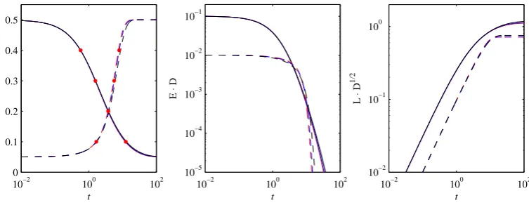
Figure 2 shows how hxi, E and L vary as functions of time, for the three values
D = 0.01, 0.02, 0.04. Forhxi the movement from 0.5 to 0.05 is somewhat slower than the
reverse process, but both processes occur on a similar timescale, and both are essentially
independent of D. This is in contrast with other Fokker-Planck systems where the
magnitude of the diffusion coefficient can have a very strong influence on the equilibration
timescales [36, 37].
For E and L the equilibration is again somewhat slower for γ = 0.5 → 0.05 than the
reverse. We can further identify clear scalings E ∼ D−1 and L ∼ D−1/2. Finally, L is
greater for γ = 0.5→0.05 than the reverse. These results are all understandable in terms
of the interpretation of L as the number of statistically distinguishable states that the
PDF evolves through: First, we recall from figure 1 that γ = 0.5 → 0.05 had consistently
narrower PDFs than the reverse. Narrower PDFs means more distinguishable states,
hence larger L for γ = 0.5→ 0.05 than the reverse. The L ∼ D−1/2 scaling has the same
explanation; smaller D yields narrower PDFs, hence largerL.
9
FIG. 1: The left panel shows the result of switchingγ = 0.5→0.05, the right panel
γ = 0.05→0.5, both at fixed = 1 andD= 0.02. The initial (red) and final (blue) gamma distributions are shown as heavy lines. The four intermediate lines are when the time-dependent solutions have hxi= 0.1, 0.2, 0.3, 0.4. The arrows are a reminder of the
direction of motion, inward on the left and outward on the right.
final gamma distributions.
Figure 2 shows how hxi, E and L vary as functions of time, for the three values
D = 0.01, 0.02, 0.04. Forhxi the movement from 0.5 to 0.05 is somewhat slower than the reverse process, but both processes occur on a similar timescale, and both are essentially independent of D. This is in contrast with other Fokker-Planck systems where the magnitude of the diffusion coefficient can have a very strong influence on the equilibration timescales [36, 37].
For E and L the equilibration is again somewhat slower for γ = 0.5 → 0.05 than the reverse. We can further identify clear scalings E ∼ D−1 and L ∼ D−1/2. Finally, L is greater for γ = 0.5→ 0.05 than the reverse. These results are all understandable in terms of the interpretation of L as the number of statistically distinguishable states that the PDF evolves through: First, we recall from figure 1 that γ = 0.5 → 0.05 had consistently narrower PDFs than the reverse. Narrower PDFs means more distinguishable states, hence larger L for γ = 0.5 → 0.05 than the reverse. The L ∼ D−1/2 scaling has the same explanation; smaller Dyields narrower PDFs, hence larger L.
10−2 100 102 0
0.1 0.2 0.3 0.4 0.5
t
<x>
10−2 100 102
10−5 10−4 10−3 10−2 10−1
t
E
⋅
D
10−2 100 102
10−2 10−1 100
t
L
⋅
D
1/2
FIG. 2: The first panel showshxi as a function of time, the second panel shows E ·D (to
indicate theE ∼D−1 scaling), and the third panel showsL ·D1/2(to indicate the
L ∼D−1/2scaling). Solid lines denote γ = 0.5→0.05, dashed lines the reverse. Each solid
or dashed ‘line’ is in fact three – occasionally barely distinguishable – lines with
D= 0.01, 0.02, 0.04. The dots on thehxi curves correspond to the PDFs shown in figure
1.
The first panel in figure 3 shows the previous quantities hxi and L · D1/2, but now
plotted against each other rather than separately against time. The behaviour is exactly
as one might expect, with L growing more or less linearly with distance from the initial
position. The right panel in figure 3 shows the entropy (15), again as a function of hxi
rather than time, to emphasize the cyclic nature of the two processes. The significance is
indeed as claimed above, with more localized PDFs having smaller entropy values. Note
how γ = 0.5 → 0.05, which had the narrower PDFs, has lower entropy values than the
reverse process. Note also how reducing D by a factor of two, thereby making the PDFs
narrower, causes the entire cyclic pattern to shift downward by an essentially constant
amount.
Figure 4 shows how the standard deviation, skewness and kurtosis behave, again as
func-tions of hxi throughout the two processes. The heavy green lines also show the behaviour
that would be expected if the time-dependent PDFs were always gamma distributions
throughout their evolution. That is, if gamma distributions have hxi = γ, σ = √γD,
skewness = 2pD/γ and kurtosis = 6D/γ (settingǫ= 1), then expressed as function ofhxi
10
FIG. 2: The first panel shows hxi as a function of time, the second panel shows E ·D(to indicate the E ∼D−1 scaling), and the third panel shows L ·D1/2 (to indicate the
L ∼D−1/2 scaling). Solid lines denoteγ = 0.5→0.05, dashed lines the reverse. Each solid or dashed ‘line’ is in fact three – occasionally barely distinguishable – lines with
D= 0.01, 0.02, 0.04. The dots on the hxi curves correspond to the PDFs shown in figure 1.
plotted against each other rather than separately against time. The behaviour is exactly as one might expect, with L growing more or less linearly with distance from the initial position. The right panel in figure 3 shows the entropy (15), again as a function of hxi
rather than time, to emphasize the cyclic nature of the two processes. The significance is indeed as claimed above, with more localized PDFs having smaller entropy values. Note how γ = 0.5 → 0.05, which had the narrower PDFs, has lower entropy values than the reverse process. Note also how reducing D by a factor of two, thereby making the PDFs narrower, causes the entire cyclic pattern to shift downward by an essentially constant amount.
Figure 4 shows how the standard deviation, skewness and kurtosis behave, again as func-tions of hxi throughout the two processes. The heavy green lines also show the behaviour that would be expected if the time-dependent PDFs were always gamma distributions throughout their evolution. That is, if gamma distributions have hxi = γ, σ = √γD, skewness = 2pD/γ and kurtosis = 6D/γ (setting= 1), then expressed as function of hxi
0 0.1 0.2 0.3 0.4 0.5 0 0.2 0.4 0.6 0.8 1 1.2 0.01 0.01 0.04 0.04 <x> L ⋅ D 1/2
0 0.1 0.2 0.3 0.4 0.5
−2.5 −2 −1.5 −1 −0.5 0 0.01 0.04 <x> Entropy
FIG. 3: The left panel showsL ·D1/2, the right panel entropy, both as functions of hxi.
Solid lines denote γ= 0.5→0.05, dashed lines the reverse. Numbers besides curves
indicate D= 0.01, 0.02, 0.04. The arrows on the entropy plot are a reminder of the
direction of inward/outward motion.
0 0.1 0.2 0.3 0.4 0.5 0.2 0.4 0.6 0.8 <x> σ / D 1/2 0.01 0.04
0 0.1 0.2 0.3 0.4 0.5 0 2 4 6 8 10 <x>
Skewness / D
1/2
0.01 0.04
0 0.1 0.2 0.3 0.4 0.5 0 20 40 60 80 100 120 <x>
Kurtosis / D
0.01 0.04
FIG. 4: σ/D1/2, (skewness/D1/2) and (kurtosis/D), as functions ofhxi. Solid lines denote
γ= 0.5→0.05, dashed lines the reverse. Numbers besides curves indicate
D= 0.01, 0.02, 0.04. The heavy green curves arephxi, 2/phxiand 6/hxi, respectively,
and indicate the behaviour expected for exact gamma distributions.
we would have σ/D1/2=phxi, (skewness/√D) = 2/phxi and (kurtosis/D) = 6/hxi. As
we can see, the γ = 0.5 → 0.05 process follows these functional relationships reasonably
well (especially for skewness and kurtosis), but for γ = 0.05 → 0.5 all three quantities
deviate substantially.
11
FIG. 3: The left panel shows L ·D1/2, the right panel entropy, both as functions of hxi. Solid lines denoteγ = 0.5→0.05, dashed lines the reverse. Numbers besides curves indicate D= 0.01, 0.02, 0.04. The arrows on the entropy plot are a reminder of the
direction of inward/outward motion.
0 0.1 0.2 0.3 0.4 0.5
0 0.2 0.4 0.6 0.8 1 1.2 0.01 0.01 0.04 0.04 <x> L ⋅ D 1/2
0 0.1 0.2 0.3 0.4 0.5
−2.5 −2 −1.5 −1 −0.5 0 0.01 0.04 <x> Entropy
FIG. 3: The left panel showsL ·D1/2, the right panel entropy, both as functions of hxi.
Solid lines denote γ = 0.5→0.05, dashed lines the reverse. Numbers besides curves
indicate D= 0.01, 0.02, 0.04. The arrows on the entropy plot are a reminder of the
direction of inward/outward motion.
0 0.1 0.2 0.3 0.4 0.5 0.2 0.4 0.6 0.8 <x> σ / D 1/2 0.01 0.04
0 0.1 0.2 0.3 0.4 0.5 0 2 4 6 8 10 <x>
Skewness / D
1/2
0.01 0.04
0 0.1 0.2 0.3 0.4 0.5 0 20 40 60 80 100 120 <x>
Kurtosis / D
0.01 0.04
FIG. 4: σ/D1/2, (skewness/D1/2) and (kurtosis/D), as functions ofhxi. Solid lines denote
γ= 0.5→0.05, dashed lines the reverse. Numbers besides curves indicate
D= 0.01, 0.02, 0.04. The heavy green curves arephxi, 2/phxiand 6/hxi, respectively,
and indicate the behaviour expected for exact gamma distributions.
we would have σ/D1/2=phxi, (skewness/√D) = 2/phxi and (kurtosis/D) = 6/hxi. As
we can see, the γ = 0.5 → 0.05 process follows these functional relationships reasonably
well (especially for skewness and kurtosis), but for γ = 0.05 → 0.5 all three quantities
deviate substantially.
11
FIG. 4: σ/D1/2, (skewness/D1/2) and (kurtosis/D), as functions of hxi. Solid lines denote
γ = 0.5→0.05, dashed lines the reverse. Numbers besides curves indicate
D= 0.01, 0.02, 0.04. The heavy green curves arephxi, 2/phxi and 6/hxi, respectively, and indicate the behaviour expected for exact gamma distributions.
well (especially for skewness and kurtosis), but for γ = 0.05 → 0.5 all three quantities deviate substantially.
0 0.1 0.2 0.3 0.4 0.5 0
0.3 0.6 0.9 1.2
0.04 0.01
<x>
Difference / D
1/2
0 0.3 0.6 0.9
0 1 2 3
x
p
0 0.1 0.2 0.3
0 3 6 9
x
p
FIG. 5: The first panel shows the difference (13) between the actual PDF and the
equivalent gamma distribution, as functions ofhxi. Solid lines denoteγ= 0.5→0.05,
dashed lines the reverse, with arrows also indicating the direction of motion. The dots at
hxi= 0.3 for γ= 0.05→0.5, and hxi= 0.1 forγ = 0.5→0.05, correspond to the other
two panels: Panel 2 compares theγ= 0.05→0.5 PDF with its equivalent gamma
distribution; Panel 3 compares the γ= 0.5→0.05 PDF with its equivalent gamma
distribution. The actual PDFs in each case are solid (red), and the equivalent gamma
distributions are dashed (blue). D= 0.04 for both sets.
Further evidence of significant deviations from gamma distribution behaviour is seen in
figure 5, showing the difference (13) directly. As expected from figure 4, γ = 0.05 → 0.5
has a much greater difference than γ= 0.5→0.05. The second and third panels show how
the PDFs compare with the equivalent gamma distributions having the same hxi and σ
values as the actual PDFs at that instant. The differences are clearly visible, especially for
γ = 0.05→0.5, but also forγ = 0.5→0.05.
B. D > γ
We next consider the case D > γ, where we demonstrated above that stationary
solutions cannot exist at all, because the time-dependent PDF can only ever get closer and
closer to the gamma distribution singularity at the origin, but can never actually achieve
it. To explore what does happen in this case then, we simply repeat the above procedure,
12
FIG. 5: The first panel shows the difference (13) between the actual PDF and the equivalent gamma distribution, as functions ofhxi. Solid lines denote γ = 0.5→0.05, dashed lines the reverse, with arrows also indicating the direction of motion. The dots at
hxi= 0.3 forγ = 0.05→0.5, andhxi= 0.1 for γ = 0.5→0.05, correspond to the other two panels: Panel 2 compares the γ = 0.05→0.5 PDF with its equivalent gamma distribution; Panel 3 compares the γ = 0.5→0.05 PDF with its equivalent gamma distribution. The actual PDFs in each case are solid (red), and the equivalent gamma
distributions are dashed (blue). D= 0.04 for both sets.
the PDFs compare with the equivalent gamma distributions having the same hxi and σ
values as the actual PDFs at that instant. The differences are clearly visible, especially for
γ = 0.05→0.5, but also for γ = 0.5→0.05.
B. D > γ
We next consider the case D > γ, where we demonstrated above that stationary solutions cannot exist at all, because the time-dependent PDF can only ever get closer and closer to the gamma distribution singularity at the origin, but can never actually achieve it. To explore what does happen in this case then, we simply repeat the above procedure, except that there is now only an ‘inward’ process, and no reverse. That is, instead of
γ = 0.5 → 0.05, let us consider γ = 0.5 → 0. (Throughout this section we will also take
D= 10−3, to facilitate comparison with results in the next section. For γ = 0 of course any
10−5 10−4 10−3 10−2 10−1 100 101
102 103
0 1 3 10 30 100
300 1000
x
p
FIG. 6: The initial condition is a gamma distribution withγ= 0.5,ǫ= 1 and D= 10−3;γ
is then switched to 0, and the solution is evolved according to Eq. (3). Numbers besides
curves indicate time, from the initial condition at t= 0 to the final time 1000. The dashed
curves indicate the equivalent gamma distributions having the samehxiand σ.
except that there is now only an ‘inward’ process, and no reverse. That is, instead of
γ = 0.5→ 0.05, let us consider γ = 0.5 → 0. (Throughout this section we will also take
D= 10−3, to facilitate comparison with results in the next section. Forγ = 0 of course any
Dis greater than γ.)
Figure 6 shows the resulting PDFs, and how they approach ever closer to the origin, but
never actually achieve the x−1 blowup that would be implied by Eq. (4) for a= γ/D= 0.
The peak amplitude simply increases indefinitely, as t1/2. The widths correspondingly
also decrease; the apparent increase is an illusion caused by the logarithmic scale for x.
The dashed lines also show the equivalent gamma distributions, as before. Note how the
difference becomes increasingly noticeable; in line with the fact that the equivalent gamma
distribution is tending toward its singular behaviour ashxi decreases, but the actual PDFs
must always havep(0) = 0.
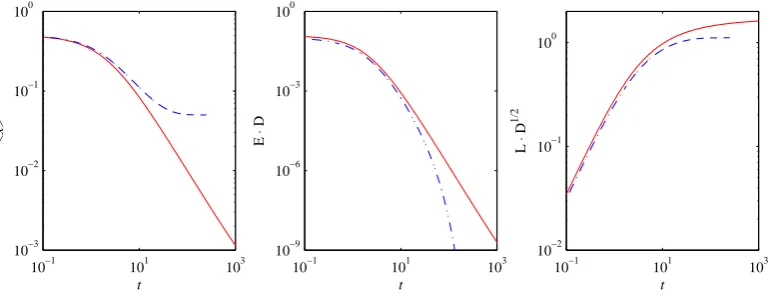
Figure 7 is the equivalent of figure 2, and directly compares γ = 0.5 → 0 here with
the previous γ = 0.5 → 0.05. We see that hxi starts out very similarly, but instead of
equilibrating to 0.05, it now tends to 0 ast−1. E again starts out similarly, but ultimately
tends to 0 much slower, as t−3 instead of exponentially. This t−3 scaling for E has an
13
FIG. 6: The initial condition is a gamma distribution with γ = 0.5, = 1 andD= 10−3;γ is then switched to 0, and the solution is evolved according to Eq. (3). Numbers besides curves indicate time, from the initial condition at t= 0 to the final time 1000. The dashed
curves indicate the equivalent gamma distributions having the samehxi and σ.
Figure 6 shows the resulting PDFs, and how they approach ever closer to the origin, but never actually achieve the x−1 blowup that would be implied by Eq. (4) for a = γ/D = 0. The peak amplitude simply increases indefinitely, as t1/2. The widths correspondingly also decrease; the apparent increase is an illusion caused by the logarithmic scale for x. The dashed lines also show the equivalent gamma distributions, as before. Note how the difference becomes increasingly noticeable; in line with the fact that the equivalent gamma distribution is tending toward its singular behaviour ashxi decreases, but the actual PDFs must always have p(0) = 0.
Figure 7 is the equivalent of figure 2, and directly compares γ = 0.5 → 0 here with the previous γ = 0.5 → 0.05. We see that hxi starts out very similarly, but instead of equilibrating to 0.05, it now tends to 0 as t−1. E again starts out similarly, but ultimately tends to 0 much slower, as t−3 instead of exponentially. This t−3 scaling for E has an interesting consequence for L, namely that L does saturate to a finite value L∞ (since
R
t−3/2dt remains bounded for t → ∞) even though the PDF itself never settles to a stationary state.
10−1 101 103 10−3 10−2 10−1 100 t <x>
10−1 101 103
10−9 10−6 10−3 100 t E ⋅ D
10−1 101 103
10−2 10−1 100 t L ⋅ D 1/2
FIG. 7: As in figure 2, the first panel showshxi, the second panel showsE ·D, and the
third panel L ·D1/2. Solid lines denoteγ = 0.5→0 forD= 10−3, dashed lines the
previous γ= 0.5→0.05 forD= 0.01. Note how the scalings ofE and LwithD are still
preserved even whenD is changed by a factor of 10.
interesting consequence for L, namely that L does saturate to a finite value L∞ (since
R
t−3/2dt remains bounded for t → ∞) even though the PDF itself never settles to a
stationary state.
Figure 8 shows entropy, σ, skewness and kurtosis, so some of the results as in figures 3
and 4. Entropy and σ are again both good measures of how narrow the PDF is, becoming
ever smaller as the peak moves toward the origin. Skewness and kurtosis seem to follow
the expected gamma distribution relationship extremely well, even though we saw before in
figure 6 that the PDFs are actually different from gamma distributions. As hxi →0, both
skewness and kurtosis thus become indefinitely large.
C. Q6= 0
Finally, we turn to the Fokker-Planck equation (11) with additive noise included, and
use it to explore the two questions that could not be addressed otherwise. First, how does
a process like γ= 0.5→0 then equilibrate to a stationary solution? Second, what does the
reverse process γ= 0→0.5 look like?
14
FIG. 7: As in figure 2, the first panel shows hxi, the second panel shows E ·D, and the third panel L ·D1/2. Solid lines denote γ = 0.5→0 forD= 10−3, dashed lines the previous γ = 0.5→0.05 for D= 0.01. Note how the scalings of E and L with D are still
preserved even when D is changed by a factor of 10.
10−3 10−2 10−1 100 −6 −5 −4 −3 −2 <x> Entropy
10−3 10−2 10−1 100 10−2 10−1 100 <x> σ / D 1/2
10−3 10−2 10−1 100 100
101 102
<x>
Skewness / D
1/2
10−3 10−2 10−1 100 101
102 103 104
<x>
Kurtosis / D
FIG. 8: Entropy, σ/D1/2, (skewness/D1/2) and (kurtosis/D), as functions ofhxi, for the
γ = 0.5→0 calculation from figure 6. The heavy green curves in the last three panels are
p
hxi, 2/phxi and 6/hxi, respectively, and indicate the behaviour expected for exact
gamma distributions.
We will keep D = 10−3 and Q= 10−5 fixed throughout this section. Since the effective
diffusion coefficients in (11) are Dx2 and Q [recall also the denominator of Eq. (12)], this
means that Qis dominant only within x ≤0.1; any stationary solutions with peaks much
beyond that are effectively pure gamma distributions.
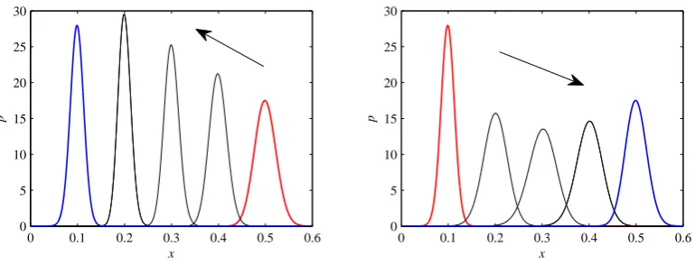
Figure 9 shows the same type of inward/outward process as before in figure 1, only
now switching γ between 0.5 and 0.1. Comparing with figure 1, we see that the dynamics
are very similar, just with all the peaks considerably narrower, which is to be expected if
D = 10−3 rather than 0.02. The only other point to note is how the final peak in the left
panel is lower than the previous peak at hxi = 0.2, which is different from figure 1, where
γ = 0.5 → 0.05 had peaks monotonically increasing throughout the entire evolution. The
reason the final peak here decreases slightly is precisely the influence of Qin this region; if
this peak is now seeing just as much diffusion from Qas from D, it is not surprising that
it spreads out somewhat more, and is correspondingly somewhat lower than a pure gamma
distribution would be.
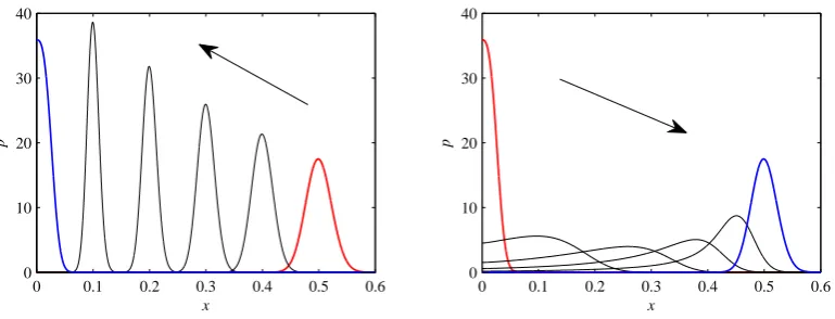
Figure 10 shows the fundamentally new case, namely switching γ between 0.5 and 0.
The inward process γ = 0.5 → 0 is again very similar to either figure 1 or 9. The only
difference to figure 6 is that the process does actually equilibrate to a stationary solution
now, as given by Eq. (12). The reverse processγ = 0→0.5 is rather different though. The
initial central peak now broadens far more than previously seen in figures 1 and 9.
FIG. 8: Entropy, σ/D1/2, (skewness/D1/2) and (kurtosis/D), as functions of hxi, for the
γ = 0.5→0 calculation from figure 6. The heavy green curves in the last three panels are
p
hxi, 2/phxi and 6/hxi, respectively, and indicate the behaviour expected for exact gamma distributions.
and 4. Entropy and σ are again both good measures of how narrow the PDF is, becoming ever smaller as the peak moves toward the origin. Skewness and kurtosis seem to follow the expected gamma distribution relationship extremely well, even though we saw before in figure 6 that the PDFs are actually different from gamma distributions. As hxi →0, both skewness and kurtosis thus become indefinitely large.
C. Q6= 0
Finally, we turn to the Fokker-Planck equation (11) with additive noise included, and use it to explore the two questions that could not be addressed otherwise. First, how does a process likeγ = 0.5→0 then equilibrate to a stationary solution? Second, what does the reverse process γ = 0→0.5 look like?
We will keep D = 10−3 and Q = 10−5 fixed throughout this section. Since the effective diffusion coefficients in (11) are Dx2 and Q [recall also the denominator of Eq. (12)], this means that Q is dominant only within x ≤ 0.1; any stationary solutions with peaks much beyond that are effectively pure gamma distributions.
Figure 9 shows the same type of inward/outward process as before in figure 1, only now switching γ between 0.5 and 0.1. Comparing with figure 1, we see that the dynamics are very similar, just with all the peaks considerably narrower, which is to be expected if
D = 10−3 rather than 0.02. The only other point to note is how the final peak in the left panel is lower than the previous peak at hxi = 0.2, which is different from figure 1, where
γ = 0.5 → 0.05 had peaks monotonically increasing throughout the entire evolution. The reason the final peak here decreases slightly is precisely the influence of Q in this region; if this peak is now seeing just as much diffusion from Q as from D, it is not surprising that it spreads out somewhat more, and is correspondingly somewhat lower than a pure gamma distribution would be.
Figure 10 shows the fundamentally new case, namely switching γ between 0.5 and 0. The inward process γ = 0.5 → 0 is again very similar to either figure 1 or 9. The only difference to figure 6 is that the process does actually equilibrate to a stationary solution now, as given by Eq. (12). The reverse process γ = 0→0.5 is rather different though. The initial central peak now broadens far more than previously seen in figures 1 and 9.
One interesting consequence of this extreme broadening for γ = 0 → 0.5 is on the total information lengthL∞. In figure 9 these values are 25 and 16, respectively, whereas in figure
0 0.1 0.2 0.3 0.4 0.5 0.6 0
5 10 15 20 25 30
x
p
0 0.1 0.2 0.3 0.4 0.5 0.6
0 5 10 15 20 25 30
x
p
FIG. 9: The left panel shows the result of switching γ= 0.5→0.1, the right panel
γ = 0.1→0.5, both at fixed ǫ= 1,D= 10−3 and Q= 10−5. The initial (red) and final
(blue) gamma distributions are shown as heavy lines. The three intermediate lines are
when the time-dependent solutions havehxi= 0.2, 0.3, 0.4. L∞= 25 on the left and 16
on the right.
One interesting consequence of this extreme broadening forγ = 0 →0.5 is on the total
information lengthL∞. In figure 9 these values are 25 and 16, respectively, whereas in figure
10 they are 35 and 9.5. That is, in both cases decreasing γ yields larger L∞ values than
increasing γ does, consistent with the peaks being narrower, and hence passing through
more statistically distinguishable states. Next, comparing 25 forγ = 0.5 → 0.1 versus 35
for γ = 0.5 → 0, this is exactly as one might expect: having the peak travel somewhat
further yields extra information length. However, comparing 16 for γ = 0.1 → 0.5 versus
9.5 for γ = 0 → 0.5 is puzzling then! The peak has further to travel, but accomplishes
it with less information length. The reason is precisely this extreme broadening, which
substantially reduces the number of distinguishable states along the way. See also [36, 37],
where the same effect was studied for Gaussian PDFs, and values of D as small as 10−7,
leading to fundamentally different scalings ofL∞ withDfor inward and outward processes.
Returning to the central question of this paper, namely how close the time-dependent
PDFs are to gamma distributions, the results for figure 9 are similar to the previous ones.
In particular, we recall that before in figure 5 we had the difference scaling as D1/2, so
16
FIG. 9: The left panel shows the result of switching γ = 0.5→0.1, the right panel
γ = 0.1→0.5, both at fixed = 1, D= 10−3 and Q= 10−5. The initial (red) and final (blue) gamma distributions are shown as heavy lines. The three intermediate lines are when the time-dependent solutions have hxi= 0.2, 0.3, 0.4. L∞= 25 on the left and 16
on the right.
increasing γ does, consistent with the peaks being narrower, and hence passing through more statistically distinguishable states. Next, comparing 25 for γ = 0.5 → 0.1 versus 35 for γ = 0.5 → 0, this is exactly as one might expect: having the peak travel somewhat further yields extra information length. However, comparing 16 for γ = 0.1 → 0.5 versus 9.5 for γ = 0 → 0.5 is puzzling then! The peak has further to travel, but accomplishes it with less information length. The reason is precisely this extreme broadening, which substantially reduces the number of distinguishable states along the way. See also [36, 37], where the same effect was studied for Gaussian PDFs, and values of D as small as 10−7, leading to fundamentally different scalings ofL∞ withD for inward and outward processes.
Returning to the central question of this paper, namely how close the time-dependent PDFs are to gamma distributions, the results for figure 9 are similar to the previous ones. In particular, we recall that before in figure 5 we had the difference scaling as D1/2, so a smaller D here means a smaller difference. These results are approaching the small D
0 0.1 0.2 0.3 0.4 0.5 0.6 0
10 20 30 40
x
p
0 0.1 0.2 0.3 0.4 0.5 0.6
0 10 20 30 40
x
p
FIG. 10: The left panel shows the result of switching γ= 0.5→0, the right panel
γ = 0→0.5, both at fixed ǫ= 1, D= 10−3 and Q= 10−5. The initial (red) and final
(blue) gamma distributions are shown as heavy lines. The four intermediate lines are when
the time-dependent solutions have hxi= 0.1, 0.2, 0.3, 0.4. L∞= 35 on the left and 9.5 on
the right.
a smaller D here means a smaller difference. These results are approaching the small D
regime where gamma distributions become very close to Gaussians anyway, which generally
remain close to Gaussian as they move.
However, for theγ = 0→ 0.5 process in figure 10, the intermediate stages do not look
much like gamma distributions. (The final equilibrium is indistinguishable from a gamma
distribution though, consistent withQbeing completely negligible for these values ofx.) For
the intermediate stages, these were found to be so different from gamma distributions that
attempting to fit a gamma distribution having the same hxi and σ made little sense; this
extreme broadening and long tail trailing behind the peak meant that both hxiand σ were
too different from the normal expectation that they should be measures of ‘peak’ and ‘width’.
Instead, we simply asked the question, which values of a and b would minimize the
quantity R|p−pbf|dx, where p is the time-dependent PDF to be fitted, and pbf is the
best-fit gamma distribution. Unlike our previous difference formula, this does not yield
simple analytic formulas for the a and b to choose, but is numerically still straightforward
to implement. Figure 11 shows the results, for two of the intermediate stages in the
17
FIG. 10: The left panel shows the result of switching γ = 0.5→0, the right panel
γ = 0 →0.5, both at fixed = 1, D= 10−3 and Q= 10−5. The initial (red) and final (blue) gamma distributions are shown as heavy lines. The four intermediate lines are when the time-dependent solutions have hxi= 0.1, 0.2, 0.3, 0.4. L∞= 35 on the left and 9.5 on
the right.
However, for the γ = 0 → 0.5 process in figure 10, the intermediate stages do not look much like gamma distributions. (The final equilibrium is indistinguishable from a gamma distribution though, consistent withQbeing completely negligible for these values ofx.) For the intermediate stages, these were found to be so different from gamma distributions that attempting to fit a gamma distribution having the same hxi and σ made little sense; this extreme broadening and long tail trailing behind the peak meant that both hxi and σ were too different from the normal expectation that they should be measures of ‘peak’ and ‘width’.
Instead, we simply asked the question, which values of a and b would minimize the quantity R |p− pbf|dx, where p is the time-dependent PDF to be fitted, and pbf is the best-fit gamma distribution. Unlike our previous difference formula, this does not yield simple analytic formulas for the a and b to choose, but is numerically still straightforward to implement. Figure 11 shows the results, for two of the intermediate stages in the
γ = 0→0.5 process. We can see that the fit is rather poor, indicating that these PDFs are
significantlydifferent from gamma distributions.
0 0.1 0.2 0.3 0.4 0.5 0.6 0
5 10 15 20
x
p
FIG. 11: The γ= 0→0.5 process as in figure 10, but now shown in more detail. The
dashed (magenta) curves are the gamma distributions that best fit the two thicker curves
at intermediate times. Note how even a ‘best-fit’ is a rather poor approximation to the
actual PDFs.
γ = 0→0.5 process. We can see that the fit is rather poor, indicating that these PDFs are
significantlydifferent from gamma distributions.
This misfit is also not caused by the inclusion ofQ; if this or any similar central peak is
evolved for either small or zeroQin the Fokker-Planck equation, the result is always similar
to here. As explained also in [36, 37], the dynamics of how central peaks move away from
the origin is simply different from how peaks already away from the origin move, regardless
of whether the final states are Gaussians as in [36, 37], or gamma distributions as here.
IV. CONCLUSION
Gamma distributions are among the most popular choices for modelling a broad range
of experimentally determined PDFs. It is often assumed that time-dependent PDFs can
then simply be modelled as gamma distributions with time-varying parametersa and b. In
this work we have demonstrated that one should be cautious with such an approach. By
numerically solving the full time-dependent Fokker-Planck equation, we found that there are
three sets of circumstances where the PDFs can differ significantly from gamma distributions:
• If D < γ, so that stationary solutions exist, butD is also sufficiently close to γ that
18
FIG. 11: Theγ = 0 →0.5 process as in figure 10, but now shown in more detail. The dashed (magenta) curves are the gamma distributions that best fit the two thicker curves
at intermediate times. Note how even a ‘best-fit’ is a rather poor approximation to the actual PDFs.
evolved for either small or zeroQin the Fokker-Planck equation, the result is always similar to here. As explained also in [36, 37], the dynamics of how central peaks move away from the origin is simply different from how peaks already away from the origin move, regardless of whether the final states are Gaussians as in [36, 37], or gamma distributions as here.
IV. CONCLUSION
Gamma distributions are among the most popular choices for modelling a broad range of experimentally determined PDFs. It is often assumed that time-dependent PDFs can then simply be modelled as gamma distributions with time-varying parameters a and b. In this work we have demonstrated that one should be cautious with such an approach. By numerically solving the full time-dependent Fokker-Planck equation, we found that there are three sets of circumstances where the PDFs can differ significantly from gamma distributions:
• If D < γ, so that stationary solutions exist, but D is also sufficiently close to γ that
a gamma distribution differs significantly from a Gaussian, then the time-dependent PDFs will also differ significantly from gamma distributions.
• IfD > γ, stationary gamma distributions do not exist at all. Instead, peaks move ever
• If the initial condition is a peak right on the origin – either as a result of adding additive noise to produce stationary solutions even forD > γ, or simply as an arbitrary initial condition – then any evolution away from the origin will differ significantly from gamma distributions. Unlike the previous two items, which become more pronounced for larger D, this effect is most clearly visible for smaller D, where the mismatch between the naturally narrower peaks and the extreme broadening seen in figure 11 becomes increasingly significant.
Future work will apply some of these ideas to fitting actual data.
V. ACKNOWLEDGEMENTS
We thank Prof Ovidiu Radulescu for motivating this work through many stimulating discussions on PDFs in biological systems.
Appendix A: Derivation of the Fokker-Planck Equations
In order to derive the Fokker-Planck equation (3) from the Langevin equation (1), it is useful to introduce a generating function Z:
Z =eiλx(t). (A1)
Then, by definition of ‘average’, the average of Z is related to the PDF,p(x, t), as
hZi=
Z
dx Z p(x, t) =
Z
dx eiλx(t)p(x, t). (A2)
Thus, we see that hZi is the Fourier transform of p(x, t). The inverse Fourier transform of
hZi then gives p(x, t):
p(x, t) = 1
2π
Z
dλ e−iλxhZi. (A3)
We note that Eq. (A3) can be written as
p(x, t) =
1 2π
Z
dλ eiλ(x−x(t))
We differentiate Z with respect to time t and use Eq. (1) to obtain
∂tZ =iλ∂txZ =iλ(γx−x2+ξ(t)x)Z =λ[γ∂λ +i∂λλ+ξ∂λ]Z, (A5)
where xZ =−i∂λZ was used. The formal solution to Eq. (A5) is
Z(t) = λ
Z
dt1 [γ∂λ+i∂λλ+ξ(t1)∂λ]Z(t1). (A6)
The average of Eq. (A5) gives
∂thZi=λ(γ∂λ+i∂λλ)hZi+λhξ(t)∂λZ(t)i. (A7)
To find hξ(t)Z(t)i, we use Eq. (A6) iteratively as follows:
hξ(t)∂λZi =
ξ(t)∂λ
λ
Z
dt1 [γ∂λ+i∂λλ+ξ(t1)∂λ]Z(t1)
= hξ(t)i∂λ
λ
Z
dt1 [γ∂λ+i∂λλ]hZ(t1)i
+∂λ
λ
Z
dt1hξ(t)ξ(t1)i∂λhZ(t1)i
= ∂λ
h
λ[D∂λhZ(t)i]
i
. (A8)
Here we used the independence of ξ(t) andZ(t1) for t1 < t, hξ(t)Z(t1)i=hξ(t)ihZ(t1)i= 0, together with Eq. (2),R0tdt1δ(t−t1) = 1/2, and hξi= 0. By substituting Eq. (A8) into Eq. (A7) we obtain
∂thZi=λ(γ∂λ+i∂λλ)hZi+λ∂λ
h
λ[D∂λhZ(t)i]
i
. (A9)
The inverse Fourier transform of Eq. (A9) then gives us
∂
∂tp(x, t) =−
∂ ∂x
h
(γx−x2)p(x, t)i+D ∂ ∂x
x ∂
∂x
h
x p(x, t)i (A10)
which is Eq. (3). Specifically, the inverse Fourier transforms of the first and last terms in Eq. (A9) are shown explicitly in the following:
1 2π
Z
dλ e−iλxh∂tZi=∂t
1 2π
Z
dλ e−iλxhZi
= ∂
∂tp(x, t), (A11) D
2π
Z
dλ e−iλxλ∂λ[λ∂λhZi] =D
∂ ∂x x ∂ ∂x h
x p(x, t)i, (A12)
where integration by parts was used twice in obtaining Eq. (A12). The additional Q∂xxp
Appendix B: Time-dependent Analytical Solutions of Eq. (3)
We begin by making the change of variables y = 1/x in Eq. (1) to obtain
dy
dt =−(γ+ξ)y+. (B1)
By using the Stratonovich calculus [2, 3, 34], the solution to Eq. (B1) is found as
y(t) = y0e−(γt+B(t))+e−(γt+B(t))
Z t
0
dt1e(γt1+B(t1)), (B2)
where y0 =y(t= 0) and B(t) =
Rt
0 dt1ξ(t1) is the Brownian motion. Therefore,
x(t) = x0e
γt+B(t) 1 +x0
Rt
0 dt1e(γt1+B(t1))
, (B3)
where x0 = x(t = 0). In Eq. (B3), eB(t) is the geometric Brownian motion while e−γt−B(t) is the geometric Brownian motion with a drift (e.g. [2]). The time integral of the latter is used in understanding stochastic processes in financial mathematics and many other areas [45, 46]. In particular, in the long time limit, its PDF can be shown to be a gamma distribution. However, this PDF of x is not particularly useful as it involves complicated summations and integrals that cannot be evaluated in closed form [45, 46].
[1] H. Risken, The Fokker-Planck Equation: Methods of Solution and Applications (Springer,
1996).
[2] F. Klebaner, Introduction to Stochastic Calculus with Applications (Imperial College Press,
2012).
[3] C. Gardiner, Stochastic Methods, 4th Ed., Chapter 4.4 (Springer, 2008).
[4] E.-W. Saw, D. Kuzzay, D. Faranda, A. Guittonneau, F. Daviaud, C. Wiertel-Gasquet, V.
Padilla and B. Dubrulle, Nat. Commun. 7:12466 doi: 10.1038/ncomms12466 (2016).
[5] E. Kim and P.H. Diamond, Phys. Rev. Lett. 88, 225002 (2002)
[6] E. Kim and P.H. Diamond, Phys. Rev. Lett. 90, 185006 (2003).
[7] E. Kim, Phys. Rev. Lett. 96, 084504 (2006).
[9] A.P.L. Newton, E. Kim and H.-L. Liu, Phys. Plasmas20, 092306 (2013).
[10] K. Srinivasan and W.R. Young, J. Atmos. Sci.69, 1633 (2012).
[11] K.M. Sayanagi, A.P. Showman and T.E. Dowling, J. Atmos. Sci.65, 12 (2008).
[12] M. Tsuchiya, A. Giuliani, M. Hashimoto, J. Erenpreisa and K. Yoshikawa, PLoS One 10,
e0128565 (2015).
[13] C. Tang and P. Bak, J. Stat. Phys. 51, 797 (1988).
[14] H.J. Jensen, Self-organized Criticality: Emergent Complex Behavior in Physical and Biological
Systems (Cambridge Univ. Press, 1998).
[15] G. Pruessner, Self-organised Criticality (Cambridge Univ. Press, 2012).
[16] G. Longo and M. Mont´evil, Progress in Biophysics and Molecular Biology: Systems Biology
and Cancer 106, 340 (2011).
[17] S.W. Flynn, H.C. Zhao, and J.R. Green, J. Chem. Phys. 141, 104107 (2014)
[18] J.W. Nichols, S.W. Flynn and J.R. Green, J. Chem. Phys. 142, 064113 (2015).
[19] M.L. Ferguson, D. Le Coq, M. Jules, S. Aymerich, O. Radulescu, N. Declerck and C.A. Royer,
PNAS 109, 155 (2012).
[20] V. Shahrezaei and P. S. Swain, PNAS 105(45) 17256 (2008).
[21] R. Thomas, L.Torre, X. Chang and S. Mehrotra, Bioinformatics 11, 576 (2010).
[22] S. Iyer-Biswas, F. Hayot, and C. Jayaprakash, Phys. Rev. E79, 031911 (2009).
[23] V. Elgart, T. Jia, A.T. Fenley and R. Kulkarni, Physical Biology8, 046001 (2011).
[24] E. Kim, H. Liu and J. Anderson, Phys. Plasmas16, 052304 (2009).
[25] E. Kim and R. Hollerbach, Phys. Rev. E 94, 052118 (2016).
[26] P. Glansdorff and I. Prigogine, Thermodynamic Theory of Structure, Stability and
Fluctua-tions (Wiley, 1971).
[27] M. Suzuki, Phys. Lett. A75, 331 (1980).
[28] M. Suzuki, Physica A105, 631 (1981).
[29] J.S. Langer, M. Baron and H.D. Miller, Phys. Rev. A.11, 1417 (1975).
[30] Y. Saito, J. Phys. Soc. Japan 61, 388 (1976).
[31] H. Hasegawa, Prog. Theor. Phys. 58, 128 (1977).
[32] B. Dennis and R. F. Costantino, Ecology69, 1200 (1988).
[33] H.-Y. Liao, B.-Q. Ai and L. Hu, Braz. J. Phys. 37, 1125 (2007).
[35] S.C. Bagui and K.L. Mehra, Am. J. Math. Stat.6, 115 (2016).
[36] E. Kim and R. Hollerbach, Phys. Rev. E 95, 022137 (2017).
[37] R. Hollerbach and E. Kim, Entropy 19, 268 (2017).
[38] L.-M. Tenk`es, R. Hollerbach and E. Kim, arXiv:1708.02789
[39] B.R. Frieden, Physics from Fisher Information (Cambridge Univ. Press, 2000).
[40] W.K. Wootters, Phys. Rev. D,23, 357 (1981).
[41] S.B. Nicholson and E. Kim, Phys. Lett. A. 379, 8388 (2015).
[42] S.B. Nicholson and E. Kim, Entropy 18, 258, e18070258 (2016).
[43] J. Heseltine and E. Kim, J. Phys. A49, 175002 (2016).
[44] E. Kim, U. Lee, J. Heseltine and R. Hollerbach, Phys. Rev. E93, 062127 (2016).
[45] J. Bertoin and M. Yor, Prob. Surveys,2, 191 (2005).