V
ALUING
Q
UALITY
Valuing quality
Laura Blow
¤and Ian Crawford
yInstitute for Fiscal Studies
June 1999
Abstract
This paper uses revealed preference restrictions and nonparametric sta-tistical methods to bound a quality-constant price series for a good that changes quality over time. Unlike the more usual hedonic regression tech-niques for estimating quality-adjusted prices, this method does not require us to observe the changing characteristics of the good or to assume a par-ticular functional relationship between these characteristics and quality. To place a bound on quality change using revealed preference conditions we as-sume that preferences are stable over time, that quality change occurs in one good or group of goods and that the direction of quality change is known.
Key Words: Cost-of-living indices, quality, GARP.
JEL Classi…cation: C43, D11.
Acknowledgements: We are grateful to Richard Blundell, Martin Browning, Sarah Tanner and seminar participants at the Institute for Fiscal Studies for helpful comments. This study was jointly funded by the Lever-hulme Trust (Grant Ref: F/386/H) and as part of the research program of the ESRC Centre for the Microeconomics of Fiscal Policy at IFS. All errors are the sole responsibility of the authors.
¤Institute for Fiscal Studies
yInstitute for Fiscal Studies and University College London.
Summary
² This paper suggests a way of using revealed preference restrictions to bound
the level of quality change for a good of interest. The model of quality
change used is the repackaging model, which assumes that quality change
acts as a multiplier on the quantity, and de‡ator on the price, of the good in
question. When consumption data violate revealed preference conditions, it
is assumed that this is because the quality of a partcular good is changing.
Quality change is calculated as the minimum quality adjustment necessary
to this good which ensures that the data are consistent with the axioms
of revealed preference. This is consistent with the maintained assumptions
that preferences are stable in quality-constant commodity space, that
viola-tions can be explained by quality change in one good, and that the quality
change is in a known direction.
² The bene…t of this technique is that a bound on quality adjustment can be
recovered without needing to know about the changing characteristics of a
good or to assume a particular functional relationship between
characteris-tics and quality, both of which are necessary for the main types of hedonic
approaches to quality measurement.
² We describe how the bound can be tightened using budget expansion paths
² The procedure is applied to simulated data with known quality change to
examine its performance. It is also applied to UK micro data on audio-visual
equipment over the period 1974 to 1996.
² Audio-visual equipment is a composite commodity which appears in the
UK Retail Prices Index. We calculate the minimum quality improvement
stable consumer preferences. We …nd that failure to account for quality
improvement in audio-visual equipment causes an upward bias in the RPI
of around 1% over the period. This means that the average annual rate of
in‡ation (January to January) over the period, which is 8.10%, is biased
1. Introduction
Economic cost-of-living indices compare the minimum cost of achieving a
refer-ence level of economic welfare across di¤erent price regimes. The notion of being
able to conduct such a comparison is based on the assumptions that consumers
behave as rational utility maximisers and that their preferences remain stable
over time. Even in the simplest of circumstances, these are strong requirements.
Quality change in goods over time complicates matters further, since a
compar-ison of the cost-of-living at di¤erent times must be based at a reference level of
quality. This means it is necessary to be able to calculate the minimum cost of
achieving a given level of welfare at a di¤erent level of quality than that which
actually prevailed at the time. This requires a theory of how quality change enters
the utility function, and hence the cost function.
It is possible to construct price indices without without making any
assump-tions on the nature of consumer behaviour (the axiomatic approach to index
numbers, for example, is concerned with constructing a price index with certain
reasonable or desirable empirical properties), but quality change poses no less of a
problem for the correct calculation of price indices than it does for cost-of-living
indices. Price indices generally compare the price of buying a given basket of
goods across di¤erent price regimes. If the quality of some good changes between
these two periods, then prices will not re‡ect the cost of buying the same (i.e.
quality-constant) good in these periods, and the price index will not be a true
re‡ection of how the cost of the …xed basket of goods has changed. To calculate
a constant price index, it is necessary to be able to calculate
quality-constant prices. The part of the price change in a good which is due to a quality
change must be stripped out of its overall price change, so that we are left with
There are two main approaches in economic theory to dealing with quality
change; the linear characteristics model originally proposed by Gorman (1956)
and developed by Lancaster (1966), and the repackaging model of Fisher and Shell
(1971) later generalised by Muellbauer (1975). Both interpret quality change as
a¤ecting the price of the quality-changing good, so that its price in any period can
be calculated at di¤erent levels of quality. This means that there is an economic
theory of quality change which is logically consistent with the method of dealing
with quality change in price indices by quality adjusting prices.
The way in which quality-adjusted prices have often been calculated in the
past is byhedonic regression techniques which parametrically estimate prices as
some function of observable characteristics of the good in question. We present
an alternative method for calculating a bound on quality change which uses the
conditions imposed by revealed preference theory. We use the repackaging model
of quality change which assumes that quality change can be represented as a
multplier on the quantity, and a de‡ator on the price, of the good in question.
When observed data violate the axioms of revealed preference, we calculate the
minimum quality adjustment necessary to the good of interest to remove the
vio-lations. This does not require us to have information on the changing
characteris-tics of the good or to make any assumptions on the exact form of the relationship
between characteristics and price, as is necessary when estimating hedonic price
indices. Our identifying assumptions are that preferences in quality-constant
com-modity space are stable, that observed violations can therefore be explained by
quality change in the good of interest, and that this quality change is in a known
direction. The assumption of stable preferences is strong, but it is one that is
often made, implicitly or explicitly, in applied microeconomic analysis. Moreover,
it is a necessary assumption for the concept of a true cost-of-living index to have
dif-…cult to make sense of the concept of quality change and of consumers’ valuation
of this quality change. We seek to explain and correct observed violations of the
axioms of revealed preference by quality change in one good (or group of goods).
This is also a strong assumption, but, given data which is not consistent with the
maximisation of a stable, well-behaved utility function, it is interesting to explore
whether there are any simple adjustments which will make the data consistent
with stable preferences, and to examine the di¤erence that these adjustments
make to the calculation of a cost-of-living or price index.
We apply our technique to simulated data with a known path of quality change
to assess how well true quality change is bounded. We also apply the technique
to the audio-visual goods section index of the Retail Prices Index (RPI) to bound
the quality change of this group of goods, and to calculate the impact that using
these quality adjusted prices has on the RPI.
The plan of this paper is as follows. In section 2 we set out more formally the
problem that quality change presents for the calculation of cost-of-living indices
and price indices. We then review the theoretical approaches to modelling quality
change in section 3. In section 4 we present a revealed preference method for
cal-culating a bound on quality change, and explain how this bound can be improved
by making use of non-parametric estimates of expenditure expansion paths.
Sec-tion 5 presents the applicaSec-tion of our method to simulated data, and secSec-tion 6
presents the empirical application to audio-visual goods. Section 7 concludes.
2. The problem of quality change for index numbers
The approach to calculating cost-of-living indices using economic theory is based
on the hypothesis of consumers as rational utility maximisers. Such a
across two price regimes. De…ning the utility function in periodtas
ut=Ut¡qt0; q1t; :::; qtK¢
we have the corresponding cost function
ct(u; p0t; p1t; :::pKt ) = min n
p0tqt :U(qt)¸u o
A cost-of-living index between two periods, r and s say, compares the cost of
achieving a given level of utility in those periods.
Csr = cr(u; p
0
r; p1r; :::pKr )
cs(u; p0s; p1s; :::pKs )
In order for this comparison to be meaningful, preferences must be stable over
time, i.e.
Ut¡qt0; qt1; :::; qKt ¢
´U¡qt0; qt1; :::; qtK ¢
Quality change poses a problem since it means that this requirement will be
violated. Suppose that good 0 is subject to quality change. Preferences over
consumption bundles will not be constant over time since a unit of good 0 in
periodris not the same as a unit of good0in periods. This means, for example,
that
Ur¡qr0; qr1; :::; qrK ¢
6
=Us¡qs0; qs1; :::; qKs ¢ for
qir =qis8i
or
cr(u; p0r; p1r; :::pKr )6=cs(u; p0s; p1s; :::pKs )forpir =pis8i
i.e. the utility derived from a consumption bundle which contains identical
phys-ical units of all goods in two di¤erent periods will not be the same, since the
quality of good 0has changed. Or the cost of achieving a given level of welfare
in two periods will not be the same even if unit prices have remained constant.
Because of this, a cost-of-living index that ignores quality change will be
where those prices represent the cost of a di¤erent quality of good. When the
qual-ity of goods is changing over time, the correct procedure should be to compare the
cost of achieving a reference level of utilityat a reference level of qualityacross
pe-riods. This requires the assumption that preferences over quality-constant goods
remains stable over time. We need to know how quality enters the utility function,
and hence cost function, to be able to base the cost-of-living index at a given level
of quality. Both the linear characteristics model and the repackaging model give
the result that quality e¤ects can be expressed purely in terms of price changes,
so that the price of good 0 in any period can be adjusted to a di¤erent level of
quality.
Price indices such as the RPI in the UK are much more commonly constructed
than true cost-of-living indices by statistical agencies. A price index measures how
the cost of buying a particular basket of goods changes over time
Psr=
p0rq
p0
sq
It is easy to see that thinking of quality change as being re‡ected in prices is also
an ideal solution to the problem of adjusting price indices to take into account
quality changes. For example, take the simple Laspeyres index
Ltt+1=
p0t+1qt
p0tqt
If the quality of good 0improves, say, between periodst andt+ 1, thenp0
t+1 is
the price of a higher quality good than was available in periodt, so that p0t+1q0t
mis-calculates the cost of buying q0
t in period t+ 1. If we think that the higher
quality of the good is re‡ected in its price level, then the price index can be
correctly calculated by stripping out the quality related change in the price of
good0 from its overall price change, i.e. we want to know what the price of good
3. Approaches to modelling quality change
Quality change has typically been approached in one of two ways in economic
theory:
1. The Linear Characteristics model originally proposed by Gorman (1956)
and developed by Lancaster (1966). This has its roots in household
pro-duction theory, which proposes that households derive utility from
non-market goods that are produced from ‘inputs’ of non-marketed goods, time etc.
The linear characteristics model is a speci…c example of this theory where
households have preferences over various characteristics, and market goods
can be described in terms of the units of di¤erent characteristics that they
embody. Quality change in a market good thus takes the form of a change
in the combination of characteristics that the good contains. If the prices
of the individual characteristics are known, then the good can be priced at
any level of quality (i.e. combination of characteristics).
2. The Repackaging model of Fisher and Shell (1971) and Muellbauer (1975).
In this model, quality change is modelled as a multiplier on the quantity of
the good in the utility function and a de‡ator on the price in the
expendi-ture function. Thus, a doubling in quality means that one physical unit of
the improved-quality good is equal to two units of the good at its original
quality.
Empirical estimation of quality-adjusted prices has tended to apply
paramet-ric regression techniques to one of the two models. In the linear characteristics
model, it must be assumed that all the relevant characterictics are observable, and
then the ‘shadow prices’ of characteristics each period are estimated by
the quality multiplier in the repackaging model, it is necessary to decide what
this quality mulitplier depends upon. The most natural hypothesis is that it
too depends on observable characteristics. The quality multiplier can then be
estimated by regressing log prices on a function of observable characteristics of
the good plus time dummies to capture the non-quality related part of price
changes. The repackaging model does not suggest a particular funtional form for
characteristics in the regression, although it is often taken to be log-linear. This
process of estimating changes in price that are to do with changes in quality via
the estimation of a parametric relationship between prices and observed
prod-uct speci…cation is generally referred to as hedonics. The assumption that the
quality multplier in the repackaging model is a function of observable
character-istics means that parametric estimation of the linear charactercharacter-istics model and
the repackaging model tend to look very similar, except for the exact functional
relationship between prices and characteristics. Despite this, it can be noted that
the two models actually derive from quite di¤erent theoretical assumptions about
what underlying preferences are de…ned over. In both cases, once the relationship
has been estimated, the good can then be priced at any base set of characteristics.
Both of the hedonic regression techniques require the assumption that the
quality of the good depends on a set of observable characteristics. In this paper,
we apply the theory of revealed preference to the repackaging model to calculate
a bound on quality adjustments to prices. Revealed preference conditions derive
from the requirement only that consumers make consistent choices. The
attrac-tion of the repackaging model is the way that quality change simply appears as
a multiplier on quantities and a de‡ator on prices. This means that it is
possi-ble to use revealed preference conditions to place a bound on quality adjustment
without needing to know about the changing characteristics of a good or to
multiplier, as is necessary with parametric estimation of the repackaging model.
In section 3.1 we outline the repackaging model in greater detail and then go on
to explain how we propose to use revealed preference conditions to calculate a
bound on quality change.
3.1. The repackaging model
Suppose that one good (good 0) is subject to quality change (we take this as
being over time, but it could equally apply to cross-sectional quality variation by,
for example, region), and that »t is an index of the quality of good 0 at time t.
The quality parameter enters directly into the utility function
ut=U¡q0t; q1t; :::; qKt ; »t¢
with
@U @» >0
i.e. higher quality yields higher utility all other things equal.
We can choose to base quality in any particular period, for example we can
set »0 = 1. Then in any subsequent period, the observed quantity of good0,q0t,
can always be adjusted to '0
t, so that
U¡qt0; q1t; :::; qtK; »t¢´U¡'0t; q1t; :::; qtK;1¢
That is, the quantity of good 0 is quality-adjusted back to some reference level
of quality normalised to one. The adjustment to q0t will depend (positively) on
»t. Intuitively, we can think about quality improvement, say, as getting a greater
quantity of the good at the old, reference quality than the actual higher-quality
quantity observed.
Call the quality adjustmentat, i.e. '0t =atq0t so
Corresponding to the utility function is a cost functionc¡u; p0
t; p1t; :::; pKt ; »t¢.
In a similar fashion, the price p0
t can be adjusted (to½0t) so that
c¡u; p0t; p1t; :::; pKt ; »t¢´c¡u; ½0t; p1t; :::; pKt ;1 ¢ Now, since min K X k=0
pktqkt s:t: u=U¡atq0t; q1t; :::; qKt ¢
can always be written as
minp
0
t
at ¡
atqt0¢+ K X
k=1
pktqkt s:t: u=U¡atq0t; q1t; :::; qtK¢
it follows that½0
t =p0t=at, i.e.
c¡u; ½0t; p1t; :::; pKt ¢ ´c µ u;p 0 t
at; p
1
t; :::; pKt ¶
Because the observed quantity purchased,q0
t, is actually likeatqt0units of the
good at its period0quality, the observed price for a current-quality unit,p0t, must
similarly translate into a price ofp0t=atfor the good at its reference quality. This
means that the budget constraint is not violated by this transformation, since
p0t
at ¡
atqt0¢=p0tqt0
In its most general form, the quality adjustmentatmay depend on the utility
levelutand/or on the quantities consumed of the di¤erent goodsqt(which we can
also normalise to one, so that all comparisons are relative to the period 0base)
as well as on the quality index»t. That is to say, a quality improvement is like
getting more of the current good at its old quality, but exactly how much more
may depend on the consumer’s utility level and combination of goods consumed.
Muellbauer (1975) shows that if the quality adjustment depends onut and qt as
well as on»t, thenat=f(ut;qt; »t), i.e.
and
c¡u; p0t; p1t; :::; pKt ; »t¢´c µ
u; p
0
t
f(ut;qt; »t)p
0
t; p1t; :::; pKt ;1 ¶
If the quality adjustment depends only on»t, thenat is a function of»t alone.
In summary, when the good 0 is subject to quality change, and the utility
function takes the form
ut=U¡q0t; q1t; :::; qKt ; »t¢
then, even when this preference structure is stable over time, preferences over
¡
q0
t; qt1; :::; qtK ¢
alone (i.e. ignoring quality change) are not stable over time. The
repackaging model allows us to write the utility function in terms of
quality-constant goods,¡atq0t; q1t; :::; qtK
¢, or the cost function in terms of quality-constant
prices, and, if we are willing to assume that these preferences are stable over time,
then we can, in theory, construct a quality-constant cost-of-living index.
4. A revealed preference approach to calculating quality change
In this section, we outline our proposed method for using the axioms of revealed
preference theory for calculating quality-adjusted prices.
Throughout this paper we use the following de…nitions and notation, following
Varian (1982).
² qt is directly revealed preferred toq, written qtR0q, ifp0tqt¸p0tq
² qt is directly revealed strictly preferred toq, writtenqtP0q, ifp0tqt>p0tq
² qtis revealed preferred toq, writtenqtRq, ifp0tqt¸pt0qs,p0sqs¸p0sqr,...,p0mqm¸
p0mq, for some sequence of observations(qt; qs; :::;qm)
² qt is revealed strictly preferred toq, writtenqtPq, if there exist observationsqs andqmsuch that qtRqs; qsP0qm; qmRq
² Data is said to satisfy the Generalised Axiom of Revealed Preference (GARP) if
GARP restrictions can only be applied to choices generated from a stable
utility function. Therefore, when good0 is subject to quality change, we cannot
apply GARP restrictions to observed choices¡qt0; qt1; :::; qKt ¢given observed prices
¡
p0t; p1t; :::; pKt ¢over time. Indeed, we may expect to …nd that observed choices
vi-olate GARP. The repackaging model supposes that the consumer’s maximisation
problem can be rewritten as
maxU¡atqt0;qKt ¢ s:t: p 0 t at ¡
atq0t ¢
+pKt 0qKt =Mt
where qKt denotes the vector of all goods except good 0, qKt = ¡qt1; :::; qtK¢,
and pK
t denotes the corresponding prices. Assuming that the utility function
U¡atq0t;qKt ¢
is stable over time, then GARP restrictions do apply to
quality-adjusted data©¡atqt0; q1t; :::; qtK¢;¡p0t=at; p1t; :::; pKt ¢ª.
The question we ask is, given observed choices which violate GARP, can we
…nd a quality-adjusted data set©¡atq0t; q1t; :::; qtK ¢
;¡p0
t=at; p1t; :::; pKt ¢ª
which does
pass GARP? This method allows us to use the conditions that GARP impose to
recover a lower bound for the value of quality changeat.
Take a two period example to illustrate, where we normalise quality to 1in
period0, so that a0= 1. Suppose we observe a GARP violation
p00q0>p00q1andp01q1>p01q0 (4.1)
What we really want to know is whether the quality-adjusted data pass GARP,
i.e. whether
p00q0 7p00¡a1q10¢+pK00qK1 (4.2)
and
p01
a1
¡
a1q01¢+pK10qK1 7 p 0 1
a1q 0
Suppose we assume that quality is increasing, soa1>1 (naturally, the same
principles can be applied if we instead assume quality has deteriorated, so that
0< a1<1). This gives the following relationship between equations 4.1, 4.2 and
4.3:
p00q0 > p00q1 (4.4)
)
p00q0 ? p00
¡
a1q10
¢
+pK00qK1
since
p00
¡
a1q10
¢
+pK00qK1 >p00q1
i.e. nothing is revealed about preferences over q0and ¡a1q01;qK1¢from this
equa-tion.
In addition
p01q1 > p01q0 (4.5)
)
p01
a1
¡
a1q01¢+pK10qK1 > p 0 1
a1q 0
0+pK10qK0
since
p01 a1q
0
0+pK10qK0 <p01q0
and, of course
p01
a1
¡
a1q01
¢
+pK1qK1 =p01q1
i.e. assuming that quality is improving, then this equation does tell us something
about preferences overq0 and¡a1q10;qK1
¢.
This is intuitively obvious. Since we are assuming a quality improvement so
thata1q01> q10, then ifq1is revealed preferred toq0even in the quality unadjusted
account. But ifq0P0q1, then we might expect this relationship to change when
we account for the fact that good0is of a higher quality in period 1than period
0.
Since we know from equation 4.5 that¡a1q10;qK1
¢
P0q0, in order to make the
data pass GARP, we need to …nd ana1 large enough to give
p00q0 < p00¡a1q10¢+pK00qK1
So the lower bound ona1 is1
a1¸ p
0
0q0¡pK00qK1
p0 0q10
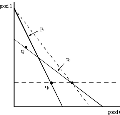
This method of quality adjustment is illustrated in …gure 4.1 for a two good
case. The observed choicesq0andq1violate GARP. We need to redraw the period
1 choice in period 0quality space. This multiplies the quantity and reduces the
price of the0thgood in period1. The points where the period1 choices in period
0quality terms can lie are along a horizontal line through q1, as indicated by the
horizontal dotted line. The dashed line to the right of the original period1budget
constraint indicates the minimum amount of quality improvement necessary for
these choices to satisfy GARP. This just places the adjusted period1 bundle on
the period0 budget constraint.
The problem with this technique, as pointed out, for example, by Varian
(1982), is that observed data often lacks the power to invoke GARP. This is
because real incomes tend to grow over time while relative prices exhibit small
variations, and so budget lines can fail to cross. This is illustrated below in …gure
1Note that the choice of time base is irrelevant. If we instead based quality in period
1and looked for an 0< a0 <1, we will again …nd that p01q1 >p01q0 )q1P0¡a0q00;qK0
¢
so we need to …nd ana0 su¢ciently small to give
p00q0< p 0 0
a0q 0
1+pK00qK1 (4.6)
Figure 4.1: Quality adjusting data using GARP — a two good, two period ex-ample.
.
.
good 0 good 1
q0
q1
p0
p1
.
4.2 by the consumption choicesq0and q1on the solid budget lines. With data
that looks like this, there is no possibility of a GARP violation, and any amount
of quality improvement would still allow the data to pass GARP.
4.1. Improving the bound
We can improve the information we have in data at arbitrary total expenditure
levels by using a method similar to one proposed by Blundell, Browning and
Crawford (1998) designed to help improve the power of tests of GARP. This
involves the non-parametric estimation, from micro data, of budget expansion
paths, which show how consumer demand changes as total expenditure changes
in a given price regime. E¤ectively, the budget constraint can be moved in or out
to any desired point.
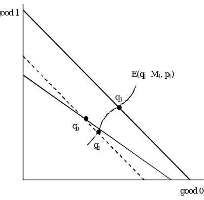
Figure 4.2: Failure of GARP to provide quality-change bounds from raw data, and using the expansion path to improve the bound.
.
good 0 good 1
q0
q1
.
.
q1E(q1³M1, p1)
testing whether the unadjusted data pass GARP and for calculating a quality
adjustment to ensure that the data does pass GARP.
Proposition 4.1. If p0tqt = p0tqr and p0rqr · p0rqt and all goods are normal, then anywhere on the periodtexpansion path passes GARP with the choice qr.
Proof.
(1) Suppose we move out along the period t expansion path from qt to eqt, so
p0tqet>p0tqt. Since all goods are normal,p0reqt>p0rqt, so
p0teqt >p0tqr; p0rqr <p0rqet
which passes GARP.
(2) Similarly, if we move in fromqtto qtthenpt0qt<p0tqtand, given normality,
p0
rqt<p0rqt, so
p0tqt <p0tqr; p0rqr ?p0rqt
which also passes GARP.
What this means, returning to the two period example, is that if we set
a¤ordable, so that
M1 ¡=p01q1¢=p01q0
and we …nd that these choices satisfy GARP, then, if we are willing to assume
that all goods are normal (which we can test for a given data set), we know that
anywhere on the period1 expansion path passes withq0.
This technique is illustrated in …gure 4.2. This shows the expansion path
giving choices of consumption bundle under price regimep1 for any level of total
expenditure M1, denotedE(q1jM1;p1). The dotted line indicates the level of
total expenditure in period 1 which would just make q0a¤ordable. The bundle
q1shows the period1 choice at this level of expenditure. In this illustration, the
choicesq0and q1constitute a violation of GARP.
Proposition 1 helps us to quality-correct the data in the following way.
Sup-pose we setM1 =p01q0and …nd that the data violate GARP, so that
M1 = p01q0
M0 > p00q1
We want to …nd the minimum quality improvement, say, that ensures the data
pass GARP. By increasing a1 and moving in along period1 expansion path we
can keep
c
M1 = p 0 1
a1q 0
0+pK10qK0
so we know that if we can …nd a point where
M0·p00
¡
a1bq10
¢
+pK00bqK1
(where qb0
1 and bqK1 denote choices given total budget Mc1) then this value of a1
will ensure that everywhere along the period1expansion path passes with q0.
Proposition 4.2. If all goods are normal, the smallest such value fora1will be
whereMc1= p 0 1
a1q 0
0+pK10qK0 andM0=p00
¡
a1bq10
¢
Proof.
(1) Suppose we …nd ana1such that
M1= p 0 1
a1q 0
0+pK10qK0 ; M0 < p00
¡
a1q01
¢
+pK00qK1
(2) We can then reduce a1to the point where
M1< p 0 1
e
a1q 0
0+pK10qK0 ; M0 =p00
¡ e
a1q01
¢
+pK00qK1
(3) From this point we can move out along the period 1 expansion path to Mf1
where
f
M1= p 0 1
e
a1q 0
0+pK1 0qK0 ; M0< p00
¡ e
a1qe01
¢
+pK00eqK1
sinceMf1> M1and therefore, assuming normality,eq1i ¸qi18i with the inequality
being strict for at least one good. Therefore we have another ea1< a1which still
ensures non-violation of GARP.
The next question is whether we can be sure that such a value ofa1will always
exist. The answer to this is yes, and is explained below.
Proposition 4.3. When M1 = p01q0 and M0 > p00q1 there will always exist a
value ofa1 such thatMc1= p 0 1
a1q 0
0 +pK10qK0 andM0=p00
¡
a1bq10
¢
+pK00bqK1 .
Proof.
(1) Everywhere on the period 1 expansion path is associated with a value of a1
which comes from setting
M1 = p 0 1
a1q 0
0+pK10qK0
Call thisa1X, so
a1X = p
0 1q00
M1¡pK1 0qK0
(4.7)
(2) Similarly, there is a value fora1 givenM1which comes from setting
M0=p00¡a1q10¢+pK00qK1
call thisa1Y, so
a1Y = M0¡p K
0 qK1
p0 0q01
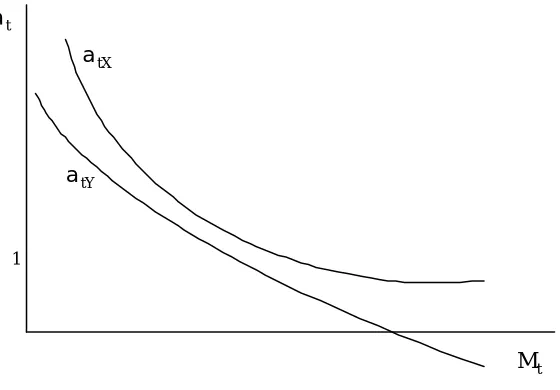
(3) Therefore, we are looking for the value of M1at which a1X=a1Y.
(4) Since the raw data violates GARP, we know that when a1X = 1, M0 >
p0
0q10+pK00qK1 so, from equation 4.8, a1Y > 1, i.e. a1X lies below a1Y at this
point. Call this point on the period1expansion path Mf1(=p01q0).
(5) Inspection of equation 4.7 shows that a1X ! 1 as M1!pK10qK0 (call this
value of the period1 budget M1). Similarly, equation 4.8 shows that a1Y ! 1
asM1!0
(6) Equation 4.7 also shows thata1X!0 asM1! 1. Equation 4.8 shows that
a1Y = 0 whenpK00q1K =M0(call the value ofM1where this occurs M1).
(7) Steps (4) and (5) imply thata1X and a1Y must intersect somewhere between
M1andMf1wherea1X =a1Y >1, and steps (4) and (6) imply thata1X and a1Y
must intersect somewhere betweenMf1andM1 where0< a1X =a1Y <1.
Therefore, when the data violate GARP there will be both a quality
improve-ment and a quality deterioration adjustimprove-ment that will …x the rejection. Although,
in the examples, we have only illustrated quality improvements, exactly the same
principles apply to quality deteriorations since they are, after all, simply di¤erent
values for a. Because, when the data violate GARP, the nature of the functions
aX and aY means that there will always be a choice of quality adjustment, we
will have to make ana prioriassumption on the direction of quality change that
we are expecting, for example in the case of computers it would be reasonable to
say we think quality has been improving.
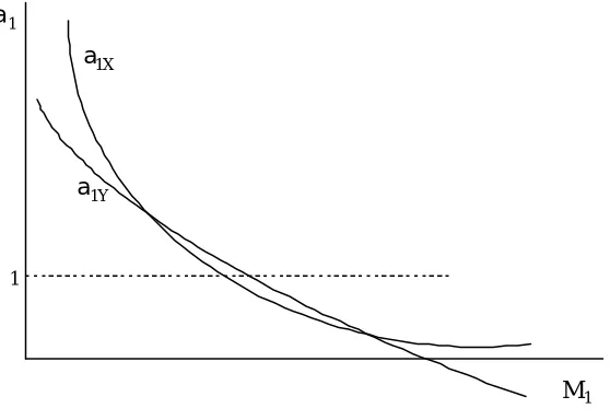
In addition, in our application, we always …nd that there is a unique value for
a1X =a1Y >1 and a unique value for0 < a1X =a1Y <1. A su¢cient condition
for uniqueness is that botha1X and a1Y are convex to the origin with respect to
M1 (for positive values ofa1, which is the only area we are interested in). This
is illustrated in …gure 4.3.
Equation 4.7 shows that, if all goods are normal, then a1X is convex (i.e.
@a1X=@M1< 0 and@2a1X=@M12> 0). If all goods are normal, then we can be
Figure 4.3: Graphical representation of calculation of quality adjustment when the raw data fail GARP.
M1
a1
a1Y a1X
1
the second derivatives ofq1with respect toM1. For example, if these are all zero,
then that is su¢cient for convexity (but it is not necessary).
4.2. More than two periods
So far, we have illustrated our technique of placing a bound on quality change
using only two periods. In practice, we will probably want to calculate the quality
change of a good over a longer time period. When there are more than two
periods, we calculate a chronological set of quality adjustments in the following
way. First, we decide on the direction of quality change we are looking for, so that
whenever there is a violation of GARP, we always choose the quality-improving
adjustment or always choose the quality-deteriorating adjustment. Suppose we
have decided on quality improvement for example, then we assume that once
quality has improved it must remain at at least that level from that time onwards.
The process is given in the following algorithm:
Inputs:
A set of quality inclusive pricesfp0;p1; ::;pTg.
A set of budget expansion pathsfE(q0jp0; M); E(q1jp1; M); :::; E(qTjpT; M)g
whereqt is(K+ 1£1).
Output:
A set of quality adjustment factorsA=f1; a1; :::; aTg.
Algorithm:
1) SetB=f0;1; :::; Tg; A=?; D=?
2) Setb= inffBg; C=B=b
3) Computeqt=E(qtjpt; Mb)andqb=E(qbjpb; Mb)8t2C
4) Ifp0bqb>pb0qtgoto (5), otherwise eat = 1, goto (6).
5) Computeeatand Mftsuch that
e
at=¡p0tq0b ¢
=³Mft¡pKt 0qKb ´
=¡M0¡pKb0eqKt ¢
=¡p0beqt0¢
where eqt=E ³
qtjpt;Mft ´
: 6) Seteat= supfeat;easg 8s < t
7) SetAeb=eat:SetD=D[b: Set B=B=D:
8) Ifb6=T goto (2), otherwise goto (9). 9) Reset B=f0;1; :::; Tg
10)Aeb= n³
infnAeb¡1
o´ e
aij8eai2Aeb o
11)A=ninfnAeb o
j8Aeb o
[1
12) Stop.
Let us assume we are looking for quality improvements. The algorithm
be-gins by comparing periods1 toT in turn to period0(our reference quality level
period in which quality is normalised to 1) and calculates the quality minimum
adjustment whenever GARP is violated. Since we are assuming that a quality
impovement can never be reversed, we then calculate a path of quality
adjust-ments from these results which sets each period’s quality adjustment equal to the
maximum of what the comparison with period0 tells us, and the highest quality
adjustment calculated for preceeding periods. For example, suppose that we have
periods0 to4, and the comparison of periods 1 to 4 with period 0 gives us this
set of values forat=a0 of 1.5, 1.2, 5, 1. Then the path of quality change is reset
to 1.5, 1.5, 5, 5. This is saved as the set Ae0 and the algorithm moves on to use
a path of quality improvement relative to period 1’s quality which is stored in
e
A1, and so on until the …nal comparison between periods T¡1 and T. At the
end, all of these quality adjustment paths are re-based, recursively to the period
1 reference quality. For example, using our illustration, suppose we found that,
compared to period 1, quality in periods 2,3 and4 was 2, 3, 3. Then, since we
know from the previous comparison of period 1 to period 0, that period 1is at
least 1.5 times better than period0, this translates into quality in periods2 to
4 compared to period 0 of 3, 4.5, 4.5. Then, we must take the maximum of the
necessary adjustments from the comparisons with period0 and with period1 —
i.e the comparison with period1 told us that period3 is at least 4.5 times better
than period0, but the direct comparison with period0told us that period3must
be at least 5 times better than period0, so we must take 5 as the value of quality
improvement. This rede…nesAe1 asf1:5;3;5;5g. The algorithm carries out this
process for all periods to give us the setA, which, when ordered from the smallest
to the largest element gives the …nal path of quality change.
This gives the intuition behind the quality-adjusting process, but it needs a
slight modi…cation for the following reason. At the end of the …rst iteration,
for example, we know that everywhere on the expansion paths for periods 1 to
T passes GARP with q0. We also know that for a period that initially failed
GARP with period0, we calculated the minimum quality improvement necessary
to make that period pass with period 0. Therefore, we know that any further
quality adjustments to that period later on in the process will not introduce
violations with period 0. However, if a period initially passed with period 0, its
price may be adjusted later on in the process, and we cannot be sure that this will
not introduce a violation between this period and period0. To see this, consider
period0. Since the data passes GARP, we have
Mt = p0tq0
M0 · p00qt
with, therefore, atY lying below atX when atX = 1 and whenM0<p00qt (when
M0 =p00qt thenatY = 1 when atX = 1). We know that the adjusted data will
violate GARP whenever atY > atX, and we cannot be sure that this will not
happen if periodtis quality adjusted so thatatX >1. The data could look like
that in …gure 4.4, so that settingatanywhere betweenbatand eatwould introduce
a GARP violation. Or it could look like that in …gure 4.5 (or atX could just be
tangent toatY at some point, or could cutatY when atX <1) in which case any
amount of quality improvement would still leave the data satisfying GARP.
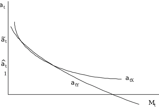
Figure 4.4: The case where quality adjustments can introduce GARP violations when the raw data pass GARP.
Mt at
atY atX
1
at a~t
^
The same point obviously applies to each iteration of the procedure as each
Figure 4.5: The case where any amount of quality adjustment still leaves the data passing GARP.
Mt at
atY atX
1
adjustment procedure, we need to recheck the data to see whether any such
violations have been introduced. If they have, then we need to reiterate the
quality adjustment procedure until all such violations are eliminated. We know
that this cannot continue inde…nitely, since there are a …nite number of bilateral
comparisons between periods, and, once a violation between two periods has been
corrected, violations will never be reintroduced by further quality improvements.
4.3. The nature of the quality adjustment function
If the quality adjustment to prices is a function ofutandqtas well as of the quality
parameter»t, then we might expect to …nd a di¤erent set of quality adjustments
depending on which part of the expenditure distribution is chosen for the base
bundle, since ut and qt will vary with total expenditure (if we assume everyone
has identical preferences, then variations inut and qt come only from variations
in Mt). In our empirical application, we calculate the quality adjustment using
di¤erent points of the expenditure distribution as the base bundle to see whether
5. Simulations
To get some idea of the power of these techniques, we …rst simulate demand data
with known quality change and apply the algorithm described above. In general
the bound on the quality change we are able to recover will, for a given true
quality change, depend upon the evolution of relative prices over time. It is,
for example, relatively easy to construct an example — typically with improving
quality and an even more rapidly increasing relative price for the a¤ected good —
in which GARP restrictions can be used to bound the true quality change quite
closely. Equally it is easy to construct an example in which GARP restrictions
provide no information. In this section we report the results of three di¤erent
simulations in which we apply the ideas described above to randomised processes
for relative prices for a given quality change scenario. We then assess how well
the procedure does compared to the known quality change. In each we use the
following CES model
max ut = "
¡
atqt0¢b+ K X
k=1
³
qtk ´b#1b
s:t: Mt = K X
k=0
pktqtk
where we setb= 0:5 and where the quality parameter on the0th good in period
t is at. We setK+ 1 = 10and T + 1 = 21 and we alter the quality of the 0th
good in each period according to three scenarios:
1. Exponential quality improvement.
2. Logistic quality improvement.
For each scenario we calculate demands given prices and compute the revealed
preference lower bound on the quality adjustment term. We repeat this 1000
times, each time generating a(10£21) matrix of relative prices according to
pt=®tpt¡1+ut
where the starting values are ones, the errors are uniformly distributed on the
unit interval and the vector®tis uniformly distributed on the range 0.9 to 1. We
then take the simulated prices for the quality-improving good, let us relabel them
aspb0t, and replace them with the quality-inclusive prices that would be observed
in practice. We allow for some randomness in the relationship between quality
and price by calculating the quality-inclusive price according to the following
relationship
lnpt = lnpb0t + ln (at°t)
where °t is uniformly distributed over the range 0.95 to 1.05. The quality
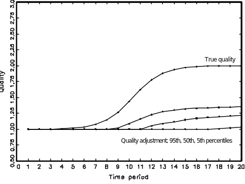
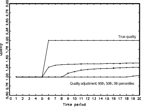
improvement held constant over repetitions. The following …gures illustrate the
true quality time series for the 0th good and the revealed preference bound at
the 5th, 50th and 95th percentiles of its distribution. The idea is to see how well
we do 90% of the time.
In each …gure the upper line is the time series for the true quality change.
Compared to the true quality change, in all cases the (median) lower bound
provided by GARP restrictions is probably quite poor. The GARP-based method
manages to pick up at least some of the quality variation for all scenarios, and for
the logistic and discrete models, where the quality change levels o¤ over time, 90%
of the simulations recover up to around one third of the improvement by the end
of the period. Nevertheless this can only be interpreted as the cost of abandoning
parametric methods if we assume that the chosen parametric method recovered
Figure 5.1: Exponential quality improvement
True quality
Quality adjustment; 95th, 50th, 5th percentiles
Figure 5.2: Logistic quality improvement
True quality
Figure 5.3: Discrete quality improvement
Quality adjustment; 95th, 50th, 5th percentiles True quality
here), or complete knowledge of the underlying data generating process (other
than the unknown quality parameter in each period), it is not clear how a usable
parametric method could be formulated. A numerical approach to calculating
the quality adjustment factor, for example, could only be implemented if the
investigator knew that preferences were CES with parameter b= 0:5. Without
this sort of insight the usual practice of using Marshallian demand curves to make
inferences regarding the appropriate functional form cannot work in this context
since if the observed data (p;q) violate GARP there exists no functional form
which is consistent with a well-behaved utility function which takes observed q
as its argument.
6. Empirical Application
We now apply the procedure to UK data on audio-visual equipment. This is a
section index of the Retail Prices Index and contains television sets, radios, audio
The bulk of the goods in this category have probably been subject to quality
improvement over the period studied, which is 1974 to 1996. The aim is to use
the techniques we have outlined to place a lower bound on the average quality
improvement of this bundle of goods over the period which will ensure that the
entire data set passes GARP. We assume that the direction of quality change is
upwards.
6.1. Data
The indices calculated in this paper use information on price movements from
the section indices of the retail price index for the period 1974 to 1996, and
cor-respondingly grouped household expenditure data from the Family Expenditure
Surveys (FES) from 1974 to 1996. The FES is an annual random cross section
survey of around 7,000 households (this represents a response rate of around
70%). The FES records data on household structure, employment, income and
the spending over the course of a two week diary period. All members of
partici-pating households over the age of 16 are asked to complete a spending diary. In
the FES the information is aggregated to the household level and averaged across
the two week period to give weekly expenditure …gures for over 300 di¤erent goods
and services.
We group the data into the thirteen non-housing RPI group index level: food,
catering, alcoholic drink, tobacco, fuel and light, household goods, household
ser-vices, clothing and footwear, personal goods and serser-vices, motoring expenditure,
fares and other travel costs, leisure goods and leisure services. Finally we remove
audio-visual equipment from leisure services and create a fourteenth category for
it. The prices we use are the corresponding RPI group price indices for the other
twelve groups, the RPI section index for audio-visual equipment and we
weight data and section indices for that group. Since the demand data from each
year of FES is collected throughout the year (except for a couple of weeks around
Christmas) we also average the prices within the year. Audio-visual equipment
carries a weight of 7/1000 in 1996.
6.2. Estimation
We estimate the budget expansion paths we require to improve the quality bound
available from the raw data by nonparametric smoothing across the cross section
of households within each month/price regime. That is, within each month, prices
are assumed constant across households and we use the cross-section variation in
total expenditure to identify the expansion path. To be more explicit denote log
expenditure for theith household bylnMiand budget share for theith household
bywij for thejth good. For each commodity j and each householdi;we assume
a Piglog structure
wij=fj(lnMi) +"ij: (6.1)
SincelnM is endogenous thenE("ijjlnMi)6= 0orE(wijjlnMi)6=fj(lnMi)
and the nonparametric estimator will not be consistent for the function of interest.
To adjust for endogeneity inlnM we use the augmented regression technique in a
semiparametric estimation framework due to Robinson (1988). We use log income
(lny) as an instrumental variable such that
lnMi=¼lnyi+vi (6.2)
withE(vjlny) = 0, and we assume that the following linear model holds
wij=fj(lnMi) +vi½j +"ij: (6.3)
We assume
Following Robinson (1988), a simple transformation of the model can be used
to give an estimator for the parameter½j. Taking expectations of (6.3) conditional
onlnMi, and subtracting from (6.3) yields
wij¡E(wijjlnM) = (vi¡E(vijlnM))½j+"ij: (6.5)
Replacing E(wijjlnM)and E(vijlnM)by their nonparametric estimators, the
parameter½j can be estimated by ordinary least squares and ispnconsistent and
asymptotically normal. The estimator forfjh(lnM)with bandwidthhis then
b
fjh(lnM) =Eh(wij¡vib½jjlnM) (6.6)
In place of the unobservable error componentv we use the …rst stage residuals
b
v= lnM¡b¼lny (6.7)
whereb¼is the least squares estimator of¼:Since¼bandb½converge atpnthe
as-ymptotic distribution forfbh(lnM)follows the distribution ofEh(wij¡vi½jjlnM).
In our empirical application we use a Nadaraya-Watson kernel regression
es-timator of thejth share equation with bandwidth h,
b
fjh(lnM) =
N¡1PiKh(lnM¡lnMl)wij
N¡1P
iKh(lnM¡lnMl)
(6.8)
with sample sizeN, whereKh(¢) =h¡1K(¢=h)is chosen to be a Gaussian kernel
weight functionK(¢), andlnMlis thel’th point in thelnMdistribution at which
we evaluate the kernel. Using the same bandwidth to estimate each fh
j(lnM)
guarantees adding up across equations.
To compute demand bundles at some given total expenditure level ³lnMf´
from these semiparametric Engel curves, we utilise our common price regime
assumption (dropping the bandwidth )
E³qjjlnM; ¼f j ´
=fbj(lnMf) Ã
f
M ¼j
!
Since the nonparametric Engel curve has a pointwise asymptotic standard error
we can evaluate the distribution of eachfbj(lnM)at a point:Brie‡y, for bandwidth
choice h and sample sizeN the variance can be well approximated at the point
lnMffor large samples by
var(fh(lnMf))'
¾2j(lnMf)cK
Nhfbh(lnMf)
where cK is a known constant and fh(lnM) is an (estimate) of the density of
lnM and
¾2j(lnMf) =N¡1X
i Ã
Kh(lnM¡lnMf)
N¡1P
iKh(lnM¡lnMf) !
(wij¡fbj(lnMf))2:
This allows us to compute the variance-covariance matrix for the expansion
paths and hence to compute standard errors for the quality adjustment by the
delta method using the prices and expenditure levels as known weights.
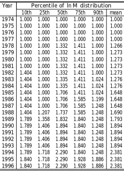
6.3. Results
We calculate the quality adjustment for di¤erent points in the within-year log
total expenditure distribution and report the results in table 6.1. The column
referring to the 1st decile, for example, reports the minimum quality adjustment
necessary for the dataset consisting of demands calculated at the 1st decile point of
the within year log total expenditure, and the group prices indices, to pass GARP.
All of the points in the total spending distribution which we have examined require
some quality adjustment in order to pass GARP and hence to be consistent with
the existence of a stable set of preferences over the period. In general the minimum
necessary quality adjustment is greatest in the middle of the distribution. By the
end of the period, for example, the dataset consisting of prices and demands at
mean log total expenditure, requires a minimum quality adjustment to
audio-visual goods of nearly 2.4. That is, by the end of this period, the observed price
around 40% of its level to be consistent with quality-constant preferences. For the
set of demands at the …rst decile point in each within-year log total expenditure
distribution to be consistent with stable preference over the period, the required
quality adjustment is about 1.8 – i.e. the price by the end must be reduced to
about 55% (at least) of its level to allow for quality changes. These di¤erences
across the spending distribution are to do with the way the expansion paths spread
out as total outlay changes and are, in general, driven by the nonhomotheticity
of the data and compositional di¤erences between the deciles. Note that, as
discussed above, even if quality change was exogenous and common in the sense
that the choice of goods and the quality improvement facing all households was
identical, the welfare derived from that change in quality (which is essentially
what we aim to bound) will vary with income, and the demands for other goods.
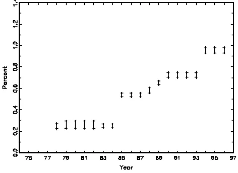
In order to calculate an adjustment in a way consistent with the RPI we
concentrate on the adjustment at the mean of the distribution. Figure 6.1 shows
the quality adjustment parameter for audio-visual equipment over the period
with 95% con…dence bounds. The con…dence bounds widen over time because
(with the exception of the …rst quality adjustment) the adjustment in period t
is dependent on the adjustment carried out in some earlier year (as described in
the algorithm). As a result variances become compounded.
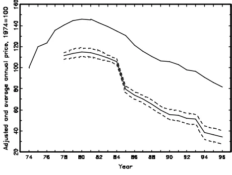
Figure 6.2 shows the annual average price index for audio-visual equipment
before and after the quality adjustment is carried out. The dashed line around
the adjusted price index is the 95% con…dence interval. If we take the published
annual index as nonstochastic (this is necessary as the sampling variance of the
RPI and its components are not published) then the di¤erence is everywhere
statistically signi…cant. Figures 6.3 and 6.4 show, respectively, the bounds on
the absolute di¤erence in index points and the percentage di¤erence between the
Table 6.1: Quality adjustment, by fractile of the within-year log total expenditure distribution, 1974=1.
Year Percentile of lnM distribution 10th 25th 50th 75th 90th mean
1974 1.000 1.000 1.000 1.000 1.000 1.000
1975 1.000 1.000 1.000 1.000 1.000 1.000
1976 1.000 1.000 1.000 1.000 1.000 1.000
1977 1.000 1.000 1.000 1.000 1.000 1.000
1978 1.000 1.000 1.332 1.411 1.000 1.266
1979 1.000 1.000 1.332 1.411 1.000 1.273
1980 1.000 1.000 1.332 1.411 1.000 1.273
1981 1.000 1.000 1.332 1.411 1.000 1.273
1982 1.404 1.000 1.332 1.411 1.000 1.273
1983 1.404 1.000 1.335 1.411 1.024 1.276
1984 1.404 1.000 1.335 1.411 1.024 1.276
1985 1.404 1.000 1.706 1.411 1.024 1.648
1986 1.404 1.000 1.706 1.585 1.199 1.648
1987 1.404 1.000 1.706 1.585 1.248 1.648
1988 1.404 1.207 1.737 1.585 1.248 1.690
1989 1.789 1.358 1.832 1.840 1.248 1.793
1990 1.789 1.406 1.894 1.840 1.248 1.894
1991 1.789 1.406 1.894 1.840 1.248 1.894
1992 1.789 1.406 1.894 1.840 1.248 1.894
1993 1.789 1.406 1.894 1.840 1.248 1.894
1994 1.789 1.718 2.290 1.840 1.248 2.381
1995 1.840 1.718 2.290 1.928 1.886 2.381
Figure 6.1: Quality adjustment and 95% condifence bounds by year, 1974=0
Figure 6.3: Di¤erence between non-housing RPI with and without quality adjust-ment, index points, 1974=100
to the calculation of the audio-visual equipment quality-constant RPI at the top
and bottom of the adjusted price series 95% con…dence interval. This indicates
that by the end of the period failure to account for quality change in
audio-visual goods alone caused an upward bias of around 6 index points, or around
1%. Over the period the annual average January to January non-housing rate of
in‡ation was 8.1%. The rate was 8.05% once the minimum adjustment for quality
improvement in audio-visual equipment was made.
7. Conclusions
This paper has suggested a way of using revealed preference restrictions to bound
the level of quality change for a good. The theoretical model used is the
repackag-ing model, which hypothesises that quality change is re‡ected by a multiplier on
the quantity of the good and a de‡ator on its price. The method used requires the
maintained assumptions that preferences in quality-constant commodity space are
stable and that the quality change is in a known direction. We explore whether
violations of revealed preference conditions can be explained by quality change
in one good (or group of goods). The main bene…t of this technique is that a
bound on quality adjustment can be recovered without needing to know about
the changing characteristics of a good or to assume a particular functional
rela-tionship between characteristics and quality — both of which are necessary for
the main types of hedonic approaches to quality measurement. We describe how
the bound can be tightened using expansion paths. The procedure is simulated
under conditions of known quality change to examine its performance. It is also
applied to UK micro data over the period 1974 to 1996, assuming that
audio-visual goods have improved in quality. Audio-audio-visual equipment is a composite
commodity which appears in the UK Retail Prices Index. We …nd that failure
re-vealed preference conditions causes an upward bias in the RPI of around 1% over
the period. This reduces the annual average January to January non-housing rate
References
[1] Blundell, R., Browning, M. & I. Crawford (1998), “Revealed preference and
non-parametric Engel curves”,University College London,Discussion Paper,
98-08.
[2] Boskin et al (1996), “Toward a more accurate measure of the cost of
liv-ing”, Final Report to the Senate Finance Commission from the Advisory
Commission to Study the Consumer Price Index .
[3] Diewert, W. E. (1976), “Exact and superlative index numbers”, Journal of
Econometrics, Vol. 4, pp. 312-36.
[4] Fisher, F.M. and K. Shell (1971), “Taste and quality change in the pure
theory of the true cost of living index” in Z. Griliches (ed) Price Indexes and
Quality Change: Studies in New Methods of Measurement, Harvard Univer-sity Press, Cambridge, M.A.
[5] Gorman, W.M. (1956), “A possible procedure for analysing quality
di¤eren-tials in the egg market”, London School of Economics, mimeo, reprinted in
Review of Economic Studies,47, 843-856 (1980).
[6] Härdle, W. (1990),Applied Non-Parametric Regression, Cambridge:
Cam-bridge University Press.
[7] Lancaster, K.J. (1966), “A New Approach to Consumer Theory”,Journal of
Political Economy,74, 132-157.
[8] Muellbauer, J. (1975), “The cost of living and taste and quality change”, Journal of Economic Theory,10, 269-283.
[9] Robinson, P.M. (1988), “Root n-consistent semiparametric regression”,
Econometrica, 56, 931-954.
[10] Prais, S.J. and Houthakker H.S. (1955), The Analysis of Family Budgets,
Cambridge: Cambridge University Press.